Analyse kinetics across mNIRS channels and intervals

Fit oxygenation kinetics (response time course) models with various parametric and non-parametric methods.

Usage

analyse_kinetics(
  data,
  nirs_channels = NULL,
  time_channel = NULL,
  method = c("response_time", "peak_slope", "monoexponential", "exponential_drift",
    "biexponential", "sigmoidal", "sigmoidal_drift"),
  start_time = NULL,
  direction = c("auto", "positive", "negative"),
  end_window = Inf,
  group_intervals = "ensemble",
  zero_time = FALSE,
  verbose = TRUE,
  ...,
  response_fraction = 0.5,
  width = NULL,
  span = NULL,
  align = c("centre", "left", "right"),
  partial = FALSE,
  na.rm = FALSE,
  use_TD = TRUE,
  shape = c("symmetric", "gompertz", "gompertz_left"),
  drift_fraction = NULL,
  fix = NULL
)

analyze_kinetics(
  data,
  nirs_channels = NULL,
  time_channel = NULL,
  method = c("response_time", "peak_slope", "monoexponential", "exponential_drift",
    "biexponential", "sigmoidal", "sigmoidal_drift"),
  start_time = NULL,
  direction = c("auto", "positive", "negative"),
  end_window = Inf,
  group_intervals = "ensemble",
  zero_time = FALSE,
  verbose = TRUE,
  ...
)

Arguments

data

A data frame, a list of data frames, or a grouped data frame of class "mnirs" containing time series data and metadata (see Details).

nirs_channels

A character vector giving the names of mNIRS columns to operate on. Must match column names in data exactly.

If NULL (default), the nirs_channels metadata attribute of data is used.

time_channel

A character string naming the time or sample column. Must match a column name in data exactly.

If NULL (default), the time_channel metadata attribute of data is used.

method

A character string specifying the kinetics analysis method. Additional arguments must be specified for each method. See Details.

"response_time": Fractional (e.g. 50%, 63.2%, 90%) response time. Additional arguments: response_fraction. See response_time().
"peak_slope": Peak rolling linear regression slope. Additional arguments: width or span, align, partial, na.rm. See peak_slope().
"monoexponential": Monoexponential curve fit via stats::nls(). Additional arguments: use_TD, fix, control. See monoexponential().
"exponential_drift": Two-phase kinetics: monoexponential primary phase with a secondary linear drift, fit via stats::nls(). Additional arguments: use_TD, drift_fraction, fix, control. See exponential_drift().
"biexponential": Two-phase kinetics: overlapping fast primary and slow secondary exponential curves fit via stats::nls(). Additional arguments: use_TD, fix, control. See biexponential().
"sigmoidal": Logistic or Gompertz-family curve fit via stats::nls(). Additional arguments: shape, fix, control. See logistic().
"sigmoidal_drift": Two-phase kinetics: Logistic or Gompertz-family primary phase with a secondary linear drift, fit via stats::nls(). Additional arguments: shape, drift_fraction, fix, control. See sigmoidal_drift().

start_time

A numeric value in units of time_channel specifying the response onset (effectively time = 0 of the fit). If NULL (default), retrieves interval_times from "mnirs" metadata, or falls back to 0 or the first positive time value (see Details).

direction

A character string specifying the response direction "positive", or "negative", or detect with "auto" (default). See Details.

end_window

A numeric value in units of time_channel specifying the window in which to look for the end of the kinetics fit; with no greater/ lesser values within end_window after the first extrema (min/max). end_window = Inf (default) returns the global extreme from the full data range (see Details).

For "biexponential", end_window bounds the fast-phase window only, and the default is 30 sec; the full model is then fit to the full data range.

group_intervals

Either "ensemble" (default) to analyse all samples of each data frame together, or a list() of integer vectors of sample (row) numbers, each analysed as a separate interval, e.g. list(trial1 = 1:10, trial2 = 11:20).

List names become interval names (interval_<n> when unnamed) (see Details).

zero_time

Logical. Default is FALSE. If TRUE, re-bases time_channel values to start from zero within each interval or group_intervals group.

verbose

Logical. TRUE (default) will display, and FALSE will silence warnings and information messages helpful for troubleshooting. Global default can be set via options(mnirs.verbose = FALSE).

...

Additional arguments passed to the underlying method function. See Details. For the stats::nls() methods (monoexponential, exponential_drift, biexponential, sigmoidal, sigmoidal_drift), control = list() can be passed to stats::nls.control(), e.g. control = list(maxiter = 200), applied globally to all channels and intervals.

response_fraction

response_time: A numeric vector in the range [0, 1] specifying the fractional response amplitude(s) to detect. Defaults to 0.5 (50% response, i.e. half-response time). Multiple values (e.g. c(0.5, 0.632)) return one coefficient row per fraction.

width

peak_slope: An integer defining the local window in number of samples around idx in which to calculate slopes. Only one of either width or span must be defined.

span

peak_slope: A numeric value defining the local window time span in units of time_channel around idx in which to calculate slopes. Only one of either width or span must be defined.

align

peak_slope: Window alignment as "centre"/"center" (the default), "left", or "right". Where "left" is forward looking, and "right" is backward looking from the current sample by the width or span.

partial

peak_slope: Logical; default is FALSE, requires local windows to have complete number of samples specified by width or span. If TRUE, processes local windows with at minimum two available samples. See Details.

na.rm

peak_slope: Logical; default is FALSE, propagates NAs to the returned vector and may return errors or warnings. If TRUE, ignores NAs and processes available valid samples within the local window. (see Details).

use_TD

monoexponential, exponential_drift, biexponential: Logical; default is TRUE, attempts to fit the model with a "time-delay" parameter TD between start_time and the response onset. If use_TD = FALSE or the fit fails (with a warning), attempts to fall back to a reduced parameter model without TD.

shape

sigmoidal, sigmoidal_drift: Character; the 4-parameter sigmoidal shape to fit. One of "symmetric" (default; inflection occurs at 50% amplitude), "gompertz" (early-inflection; 36.8% 1/e), or "gompertz_left" (late-inflection; 63.2% 1 - 1/e).

drift_fraction

exponential_drift, sigmoidal_drift: A numeric fraction of the primary amplitude in (0.5, 1) at which the linear secondary drift begins, where the primary response reaches A + drift_fraction * (B - A). Default is 0.95. Specify per-channel as a list keyed by channel name, e.g. drift_fraction = list(smo2 = 0.9). See Details.

fix

monoexponential, exponential_drift, biexponential, sigmoidal, sigmoidal_drift: An optional named list of model parameters (coefficients) to hold constant during fitting, e.g. fix = list(A = 0) fixes the starting amplitude at 0.

Fixed parameters are excluded from estimation and returned as constant. Specify per-channel as a list of lists keyed by channel name, e.g. fix = list(smo2 = list(A = 0)). See Details.

Value

A formatted table of results, with individual elements accessible as a structured list of class "mnirs_kinetics" containing:

method: The method used, e.g. "response_time".
model: A named list of model objects (per interval, per nirs_channel). For "peak_slope"; each element is an lm object. For parametric models; an nls object. For "response_time"; NULL. Models are fitted on time elapsed from start_time, so predict expects a time_channel column in newdata with adjusted units. The offset for each interval can be retrieved from coefficients$start_time.
coefficients: A data frame of coefficients with one row per nirs_channel per interval, containing interval, nirs_channels, the resolved start_time (the fit onset from which time coefficients are elapsed), and method-specific parameters. For methods with fallback options; model names the final method for each row.
data: A list of the original input data frames augmented with a *_fitted column of fitted values for each processed nirs_channel (e.g. smo2_fitted).
interval_times: A data frame with one row per interval and numeric column start_times – the resolved response onset used for fitting (the supplied start_time, else the extract_intervals() metadata, else 0 or the first positive time value) – and end_times when any interval carries an end time from the metadata.
diagnostics: A data frame of model diagnostics (n_obs, n_params, r2, adj_r2, rmse, cv_rmse, snr, aic, aicc, bic) with one row per nirs_channel per interval. n_params counts the free parameters estimated by the solver, excluding any held by fix, so a reduced-parameter fallback fit is distinguishable from a full one. n_obs and n_params need to be considered carefully when comparing fit diagnostics between models.
channel_args: A data frame of the resolved arguments used for each nirs_channel with one row per nirs_channel per interval.
warnings: A data frame of warning and error messages captured during fitting, with columns interval, nirs_channels (empty for interval-level warnings), type ("warning" or "error"), and message; zero rows when none occurred. Conditions are captured regardless of verbose, which controls console output only.
call: The matched call.

Details

Data input formats

analyse_kinetics() accepts data in multiple formats:

A single "mnirs" data frame is processed as a single interval.
A list of "mnirs" data frames: each interval is processed separately.
A grouped "mnirs" data frame, e.g. with dplyr::group_by(): the data frame is split by grouping levels and each group is processed as a separate interval.
A special case for recursive analysis: The results from analyse_kinetics() can be fed into a second call to analyse the results$coefficients table, split into data frames by nirs_channel with one row per interval (see Recursive analysis).

Specified nirs_channels (or channels retrieved from "mnirs" metadata) will be analysed and results returned as a formatted table.

Response start_time and the baseline window

start_time should be specified as the time point separating the pre-response baseline (time_channel <= start_time) from the start of the systematic response fit window (time_channel > start_time). This often corresponds to a stimulus or start/end of an intervention (e.g. start/end of an exercise interval).

For intervals extracted with extract_intervals(), start_time can be retrieved from "mnirs" metadata. Otherwise start_time defaults to 0 or the first positive time_channel value.

All methods are fitted on time elapsed from start_time, so returned time & duration coefficients are relative to response onset (e.g. start_time = 0).

For "response_time", the baseline window before start_time defines the mean starting amplitude A directly and anchors the start of the response_time parameter.
For "peak_slope", start_time anchors the start of the peak_slope_time parameter.
For "exponential"- and "sigmoidal"-family, the baseline window before start_time anchors the starting fitted amplitude A and the start of TD and MRT, or xmid parameters. (see respective method sections below).

The time-delay models ("exponential"-family with use_TD = TRUE) are flat at A before TD, so the pre-onset baseline is included in the fit and anchors A. Their reduced forms (use_TD = FALSE, or a TD fit that failed and fell back) have no such flat region and are fitted only where time_channel >= start_time.

Response direction and the fit end_window

direction is detected automatically by default as either "positive" (upward) or "negative" (downward) response, and can be overwritten manually. end_window is a time span in units of time_channel defining the end of the kinetics fitting window by locating the first extrema (peak/trough, depending on direction) with no greater/lesser values within the subsequent end_window time span. The curve fitting window extends to the end of end_window beyond the detected extrema.

For "exponential"- and "sigmoidal"-family methods, direction also constrains the sign of the fitted amplitude B - A, and the sigmoidal slope. For the "biexponential" method, direction constrains the sign of the fast-phase amplitude B - A. A fit that cannot satisfy the requested direction returns NA coefficients with a warning.

Grouping samples with group_intervals

group_intervals = "ensemble" (the default) analyses every sample of each data frame together as one interval. A list() of sample (row) numbers instead splits each data frame into one interval per group, e.g. for a 20-row data frame:

analyse_kinetics(
    data,
    method = "monoexponential",
    group_intervals = list(trial1 = 1:10, trial2 = 11:20)
)

List names become interval names; unnamed groups are interval_<n>.
Interval names are suffixed <group>_<df> (e.g. trial1_A).
For "mnirs_kinetics" results analysed recursively, the source nirs_channel is prefixed to the analysed coefficient names (e.g. smo2_slope)
Samples in no group are excluded from analysis (with a message). Samples in more than one group are allowed (with a warning).
Row-grouped intervals no longer correspond to their extract_intervals() interval_times metadata, which is dropped, so start_time falls back to the first non-negative time_channel value unless supplied explicitly (optionally per-interval, keyed by group name).
zero_time = TRUE rebases each group's time_channel to its first sample, so start_time then defaults to 0.
Per-interval arguments key by the group names (see below).

Per-channel and per-interval arguments

Arguments apply globally to all nirs_channels by default. Arguments can instead be uniquely supplied per-channel as a named list() with names matching nirs_channels. For multi-interval input (a list of data frames or a grouped data frame), a named list() can also be keyed by interval name (the list names, group keys, or interval_<n>) to supply values per-interval, and each per-interval value may itself be a per-channel list(), e.g.

analyse_kinetics(
    data,
    nirs_channels = c(o2hb, hhb),
    method = "peak_slope",
    span = list(10, o2hb = 20),
    direction = list(
        interval_1 = list(hhb = "negative", "auto"),
        interval_2 = "positive"
    )
)

The same rules apply at both levels:

A non-list value applies to every interval and channel (the default behaviour).
A list() named by interval or nirs_channels applies to those values per-interval or per-channel.
A single unnamed value in the list is the fallback applied to any unlisted intervals or channels (e.g. span = list(10, o2hb = 20) gives o2hb 20 and every other channel 10). If no unnamed fallback value in the list, unlisted intervals or channels fall back to the argument's default (i.e. NULL, or may fail with a warning).
list() names matching neither interval names nor nirs_channels are warned about and ignored.

start_time, direction, and end_window are per-channel and per-interval capable, along with the method-specific arguments except control, which is always global. fix is itself a named list() of model parameters, so a per-channel or per-interval fix is supplied as a list() of list()s keyed by channel or interval name. A plain parameter list applies everywhere:

## fix `A` at 0 for every channel
fix = list(A = 0)

## fix `A` per-channel, leaving unspecified channels free
fix = list(o2hb = list(A = 0), hhb = list(A = 5, B = 20))

## fix `A` per-interval, optionally nested per-channel
fix = list(interval_1 = list(A = 0))
fix = list(interval_1 = list(o2hb = list(A = 0)))

Triple nested list()s is janky, but it works for now!

Limitation: method itself currently only accepts a single value applied globally to all intervals and nirs_channels. So analysing channels or intervals with entirely different kinetics models must be done with independent analyse_kinetics() calls, or other iterative solutions (e.g. lapply() or purrr::map()).

method = "response_time"

Aliases: method = c("response time", "half recovery time", "half time", "HRT").

A non-parametric approach (estimated directly from the observed data without assuming a specific mathematical shape) to estimate the response time at which a signal reaches a specified fraction of its total response amplitude relative to the baseline. e.g. half-response time (response_fraction = 0.5) is the time from response onset to attain 50% of the total amplitude change and approximates the inflection point (xmid of a symmetrical sigmoid function).

response_fraction = 0.632 approximates the time constant (tau; $\tau$) parameter from a monoexponential function, or the inflection point (xmid) of an asymmetrical left-Gompertz function. response_fraction = 0.368 approximates xmid of a right-Gompertz function. This is a good fallback estimation method if parametric methods are not successfully fit.

The target response value is: fitted = A + (B - A) * response_fraction

Where A is the mean baseline value (time_channel <= start_time) and B is the first local extreme (peak or trough) value with no greater extreme values within end_window. response_value is the first observed sample where the signal is equal to or greater/lesser than the target response_fitted value. response_time is the elapsed time from start_time to response_value. See response_time() for the full algorithm and coefficients.

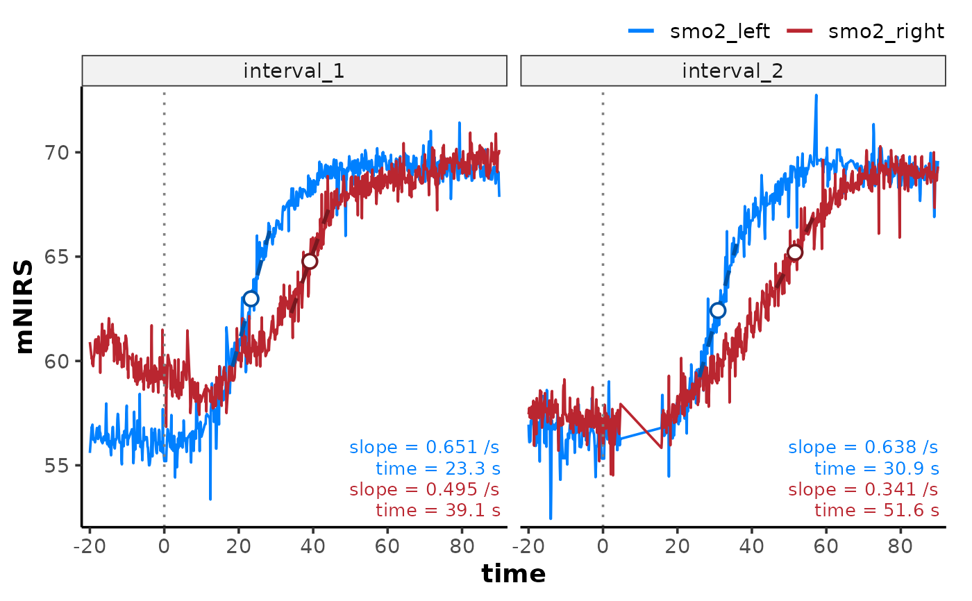
method = "peak_slope"

Aliases: method = c("peak slope", "slope", "lm").

A semi-parametric approach to estimate the maximum positive or negative local linear slope of a signal using rolling least-squares regression. The steepest local rate of change in NIRS signals can be interpreted as the moment of greatest mismatch between oxygen delivery and extraction. peak_slope_time is the time from response onset start_time to this moment of greatest mismatch.

The local window is defined by either width (number of samples) or span (in units of time_channel). See peak_slope() for window mechanics, partial-window behaviour, and the returned vector-level list.

method = "monoexponential"

Aliases: method = c("monoexp", "exponential", "exp", "tau", "MRT").

A parametric approach fitting a self-starting monoexponential function to the response curve using stats::nls() with SSmonoexponential() for either a 4-parameter (A, B, tau, TD) or 3-parameter (A, B, tau) model.

Model equations:

3-parameter: A + (B - A) * (1 - exp(-t / tau))
4-parameter: A + (B - A) * (1 - exp(-pmax(t - TD, 0) / tau))

TD is the time delay from start_time to the onset of the exponential response curve. tau is the time constant of the response. The rate constant k is the reciprocal (k = 1 / tau). The mean response time is the time sum MRT = TD + tau. See monoexponential() for the model family and SSmonoexponential() for self-start initialisation.

Any parameter may be held constant with fix, e.g. fix = list(A = 0). This excludes them from the fit optimisation procedure, and effectively reduces the function to a lower-parameter model. TD can only be fixed when use_TD = TRUE and disables the 3-parameter fallback. It is recommended to specify use_TD = FALSE rather than fix TD = 0.

method = "exponential_drift"

Aliases: method = c("exp_drift", "exp_linear", "monoexp_drift").

A parametric approach fitting a self-starting two-phase curve using stats::nls() with SSexponential_drift(). A fast monoexponential() primary response plus a slow linear secondary drift beginning near the primary asymptote.

Model equation:

A + (B - A) * (1 - exp(-pmax(t - TD, 0) / tau)) + slope_B * pmax(t - TD + tau * log(1 - drift_fraction), 0)

A, B, tau, TD, and the derived k, MRT, and HRT are as for "monoexponential". slope_B is the linear drift rate dx/dt. The drift onset is not a free estimate. drift_fraction specifies the fraction ((0.5, 1)) of the primary response amplitude where the drift begins; TD - tau * log(1 - drift_fraction) (default 0.95; TD + 3 * tau).

The excursion point texc is where the drift rate overtakes the decaying primary rate, TD + tau * log(|B - A| / (|slope_B| * tau)), floored at the drift onset, elapsed from start_time (the same frame as TD and MRT).

The drift component is kept only when the data support it. The model will fall back to "monoexponential" when the fit fails or if the total drift amplitude is below twice the fit RMSE, with a warning recorded in warnings. The model column in coefficients names the final method for each row. A hidden argument model_fallback = FALSE will override the fallback process and retain the more complex model, or return an error.

Parameters may be held constant with fix, e.g. fix = list(A = 0), as above.

method = "biexponential"

Aliases: method = c("biexp", "double exponential").

A parametric approach fitting a self-starting two-phase biexponential excursion-recovery function to the response curve using stats::nls() with SSbiexponential(). A fast primary component driving the initial excursion, and a slow secondary component recovering the response toward a stable plateau.

Model equations:

5-parameter: A + (B - A) * (1 - exp(-t / tau)) + (B2 - B) * (1 - exp(-t / tau2))
6-parameter, where ts = pmax(t - TD, 0): A + (B - A) * (1 - exp(-ts / tau)) + (B2 - B) * (1 - exp(-ts / tau2))

A is the starting value. B & tau are the asymptote and time constant of the fast response. B2 & tau2 are the asymptote and time constant of the slower response plateau (typically tau2 >> tau).

Set use_TD = TRUE (default) to specify the time-delay parameter TD. The fast-phase mean response time MRT = TD + tau is reported as for "monoexponential". See biexponential() for the model family and SSbiexponential() for self-start initialisation.

The two phases are fit sequentially.

Stage 1 fits the fast phase as a "monoexponential" on the supplied end_window window, giving A, tau, and TD (if selected).
Stage 2 fits the full model to the whole response with A, tau, and TD held within a tight range of their stage-1 values, and B, B2, tau2 free.

Secondary tau2 is floored above the primary tau, so the phases stay separated. tau2 is arbitrarily capped at ten times the fit window timespan, functionally implying the true asymptote is linear not exponential. end_window should be set to isolate the fast phase; by default resolves to 30 sec instead of Inf (recorded in channel_args).

The biexponential fit is kept only when the data support both phases. The model will fall back to "exponential_drift" when the fit fails (e.g. phases not separable), the fitted response is monotonic (no estimable excursion point texc), tau2 exceeds twice the fitted time span (a slow phase the record cannot tell from a linear drift), or the slow-phase amplitude |B2 - B| is below twice the fit RMSE.

The exponential-drift fit is in turn subject to its own fallback to "monoexponential" (see above). Each fallback is warned about and recorded in warnings. The model column in coefficients names the final method for each row. A hidden argument model_fallback = FALSE will override the fallback process and retain the more complex model, or return an error.

Parameters may be held constant with fix, e.g. fix = list(A = 0), as above.

method = "sigmoidal"

Aliases: method = c("logistic", "gompertz", "xmid").

A parametric approach fitting a self-starting 4-parameter sigmoidal function to the response curve using stats::nls() in one of three shapes.

Model equations (all 4-parameter):

shape = "symmetric" (SSlogistic()): A + (B - A) / (1 + exp(-4 * slope * (t - xmid) / (B - A)))
shape = "gompertz" (SSgompertz()): A + (B - A) * exp(-exp(-k * (t - xmid))) with k = slope * e / (B - A). Early-acceleration; inflection height fixed at A + (B - A) / e; 36.8% of the amplitude.
shape = "gompertz_left" (SSgompertz_left()): A + (B - A) * (1 - exp(-exp(k * (t - xmid)))) with k = slope * e / (B - A). Late-acceleration; inflection height fixed at A + (B - A) * (1 - 1/e); 63.2% of the amplitude.

xmid is the time from start_time to the inflection point; the steepest point of the response. slope is the response rate dx/dt at the inflection.

A "symmetric" shape is the default when no obvious asymmetry is expected. "gompertz" (right-inflection) growth is appropriate for fast-onset, slow-tail responses. "gompertz_left" for slow-onset, fast-tail responses. See logistic(), gompertz(), and gompertz_left() for the model families and SSlogistic(), SSgompertz(), and SSgompertz_left() for self-start initialisations.

Parameters may be held constant with fix, e.g. fix = list(A = 0), as above.

method = "sigmoidal_drift"

Aliases: method = c("sigmoid_drift", "sig_drift", "sig-lin", "logistic_drift", "gompertz_drift").

A parametric approach fitting a self-starting two-phase curve using stats::nls() with SSsigmoidal_drift(). A fast "sigmoidal" primary response of the given shape plus a slow linear secondary drift beginning near the primary ending asymptote.

Model equation:

S(t) + slope_B * pmax(t - onset, 0)

S(t) and A, B, xmid, and slope are as for "sigmoidal". slope_B is the linear drift rate dx/dt at the asymptote B. The drift is not a free estimate. drift_fraction specifies the fraction ((0.5, 1)) of the primary response amplitude where the drift begins (default 0.95).

The excursion point texc is where the drift rate overtakes the decaying primary rate, |S'(t)| = |slope_B|, floored at the drift onset, elapsed from start_time (the same frame as xmid).

The drift component is kept only when the data support it. The model will fall back to "sigmoidal" when the fit fails or if the total drift amplitude is below twice the fit RMSE, with a warning recorded in warnings. The model column in coefficients names the final method for each row. A hidden argument model_fallback = FALSE will override the fallback process and retain the more complex model, or return an error.

Parameters may be held constant with fix, e.g. fix = list(A = 0), as above.

Recursive analysis

An "mnirs_kinetics" result may be passed back as data to analyse how coefficients change across intervals, e.g. analyse_kinetics(result, nirs_channels = tau, time_channel = start_time, method = "peak_slope"). nirs_channels and time_channel must name coefficient columns explicitly; no metadata defaults are applied.

Time-point coefficients (response_time, peak_slope_time, TD, MRT, HRT, texc, xmid) are elapsed from each interval's start_time. When one of these is given as time_channel, start_time is added row-wise so the analysis runs on absolute time. start_time itself and duration coefficients (e.g. tau) are unchanged.

Coefficient rows from separate trials can be analysed separately with group_intervals, e.g. 20 occlusion slopes from two trials:

analyse_kinetics(
    result,
    nirs_channels = slope,
    time_channel = peak_slope_time,
    method = "monoexponential",
    group_intervals = list(trial1 = 1:10, trial2 = 11:20)
)

Examples

result <- read_mnirs(
    file_path = example_mnirs("train.red"),
    nirs_channels = c(
        smo2_left = "SmO2 unfiltered",
        smo2_right = "SmO2 unfiltered"
    ),
    time_channel = c(time = "Timestamp (seconds passed)"),
    zero_time = TRUE,
    verbose = FALSE
) |>
    resample_mnirs(method = "linear", verbose = FALSE) |>
    extract_intervals(
        group_intervals = "distinct",
        start = by_time(368, 1084),
        span = c(-20, 90),
        zero_time = TRUE,
        verbose = FALSE
    ) |>
    analyse_kinetics(
        nirs_channels = c(smo2_left, smo2_right),
        method = "peak_slope",
        span = 10,          ## 10-second rolling window
        direction = "auto", ## auto-detect slope direction
        verbose = FALSE
    )

## formatted table of results
result
#> 
#> Peak Linear Response Rate
#>     Model Coefficients:
#>     interval nirs_channels  slope intercept peak_slope_time
#> 1 interval_1     smo2_left 0.6508     47.82            23.3
#> 2 interval_1    smo2_right 0.4952     45.41            39.1
#> 3 interval_2     smo2_left 0.6376     42.71            30.9
#> 4 interval_2    smo2_right 0.3409     47.61            51.6
#> 
#> 

## coefficients are accessible from the result list
result$coefficients
#>     interval nirs_channels start_time     slope intercept   fitted
#> 1 interval_1     smo2_left          0 0.6507819  47.81776 62.98098
#> 2 interval_1    smo2_right          0 0.4952500  45.40962 64.77390
#> 3 interval_2     smo2_left          0 0.6376464  42.71328 62.41656
#> 4 interval_2    smo2_right          0 0.3409474  47.61278 65.20566
#>   peak_slope_time idx
#> 1            23.3 434
#> 2            39.1 592
#> 3            30.9 510
#> 4            51.6 717

## along with diagnostics and other returned objects
result$diagnostics
#>     interval nirs_channels n_obs n_params        r2    adj_r2      rmse
#> 1 interval_1     smo2_left   101        2 0.9036017 0.9026280 0.6197138
#> 2 interval_1    smo2_right   101        2 0.8501018 0.8485877 0.6063126
#> 3 interval_2     smo2_left   101        2 0.9043816 0.9034158 0.6044832
#> 4 interval_2    smo2_right   101        2 0.8251746 0.8234086 0.4575370
#>       cv_rmse       snr      aic     aicc      bic
#> 1 0.009839698 10.159306 195.9691 196.2165 203.8144
#> 2 0.009360447  8.242037 191.5530 191.8004 199.3983
#> 3 0.009684661 10.194586 190.9425 191.1900 198.7879
#> 4 0.007016830  7.573953 134.6823 134.9297 142.5276

## plot results
plot(result)

Analyse kinetics across mNIRS channels and intervals

Usage

Arguments

Value

Details

Data input formats

Response start_time and the baseline window

Response direction and the fit end_window

Grouping samples with group_intervals

Per-channel and per-interval arguments

method = "response_time"

method = "peak_slope"

method = "monoexponential"

method = "exponential_drift"

method = "biexponential"

method = "sigmoidal"

method = "sigmoidal_drift"

Recursive analysis

See also

Examples