Monoexponential function with 4 parameters

Calculate a four-parameter monoexponential curve.

Usage

monoexponential(t, A, B, tau, TD = NULL)

Arguments

t

A numeric vector of the predictor variable; time or sample number.

A

A numeric parameter for the starting (baseline) value of the response variable.

B

A numeric parameter for the ending (asymptote) value of the response variable.

tau

A numeric parameter for the time constant tau (\(\tau\)) of the exponential curve, in units of the predictor variable t.

TD

A numeric parameter for the time delay before the onset of exponential response, in units of the predictor variable t. If NULL (default), a 3-parameter model without time delay is used.

Value

A numeric vector of predicted values the same length as the predictor variable t.

Details

3-parameter model equation: A + (B - A) * (1 - exp(-t / tau))

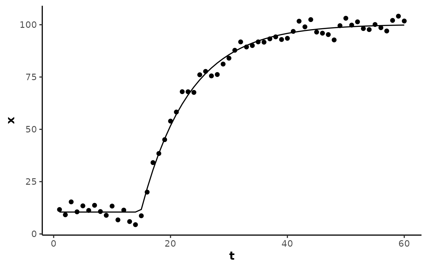
4-parameter model equation: ifelse(t <= TD, A, A + (B - A) * (1 - exp(-(t - TD) / tau)))

tau is the time constant and equal to the reciprocal of k, the rate constant (k = 1/tau).

See also

SS_monoexp()

Examples

set.seed(13)
t <- 1:60

## create an exponential curve with random noise
x <- monoexponential(t, A = 10, B = 100, tau = 8, TD = 15) + rnorm(length(t), 0, 3)
data <- data.frame(t, x)

(model <- nls(x ~ SS_monoexp4(t, A, B, tau, TD), data = data))
#> Nonlinear regression model
#>   model: x ~ SS_monoexp4(t, A, B, tau, TD)
#>    data: data
#>       A       B     tau      TD 
#>  10.461 100.233   8.313  14.884 
#>  residual sum-of-squares: 455.5
#> 
#> Number of iterations to convergence: 5 
#> Achieved convergence tolerance: 7.481e-07

y <- predict(model, data)

library(ggplot2)
ggplot(data, aes(t, x)) +
    theme_mnirs() +
    geom_point() +
    geom_line(aes(y = y))