Analysing muscle oxidative capacity with {mnirs}
2026-02-08
Source:vignettes/articles/oxcap-analysis.qmd
Introduction
I am continuing to develop the {mnirs} package for processing and analysing muscle near-infrared spectroscopy in R.
In this article, I will demonstrate how the recently added functionality can be combined to perform muscle oxidative capacity (OxCap) analysis from a repeated ischaemic occlusion protocol, while ensuring reproducibility and adhering to current gold-standard processing methods.
Tip
This article assumes basic familiarity with the {mnirs} package. For an overview and demonstration of data processing with {mnirs}, please see the package vignette Reading and Cleaning Data with {mnirs}.
Muscle oxidative capacity testing
One of the most compelling applications emerging in mNIRS research is the ability to non-invasively evaluate muscle oxidative capacity after a dynamic exercise task.
Oxidative capacity is the maximal rate at which a muscle utilises oxygen (O2) to meet the energetic demand of exercise, and is related to mitochondrial respiratory function [1].
Traditionally, OxCap assessment requires highly complex and invasive in-vitro methods such as high-resolution respirometry of biopsy tissue samples, or expensive in-vivo 31P magnetic resonance spectroscopy.
With mNIRS, muscle OxCap can be assessed non-invasively during more dynamic exercise tasks, and with lower cost and burden than traditional methods previously available.
Protocol overview
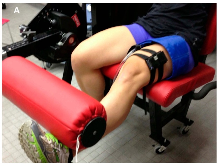
The participant is asked to perform a brief exercise task or muscle contraction stimulus to elevate the O2 demand in the target tissue, with mNIRS sensors over the peripheral muscle of interest and an occlusion cuff ready (deflated) around the proximal limb.
Immediately after the stimulus, the occlusion cuff is rapidly inflated to a supra-systolic blood pressure (e.g., 300 mmHg) to transiently stop blood flow into the distal target muscle site.
The occlusion is held for a brief period such as 5-seconds, then deflated to allow recovery to proceed. A sequence of these brief, repeated occlusions are performed at a pre-specified tempo (e.g. 5-sec occlusion, 10-sec recovery) for up to twenty repetitions (~5-minutes) until the muscle has recovered back to baseline.
During each occlusion where oxygen delivery is constrained and assumed to be zero, the rate of deoxygenation — the slope of the rise in deoxyhaeme (HHb/time; μM/sec), or decline in oxygen saturation or oxyhaeme — is interpreted to represent the rate of local muscle oxygen uptake (mV̇O2).
Immediately after the exercise task when metabolic demand is high, mV̇O2 will be elevated. It will decline at an exponential rate as recovery proceeds back to baseline. The rate constant (k, min-1) of this monoexponential curve quantifies the muscle OxCap value [3].
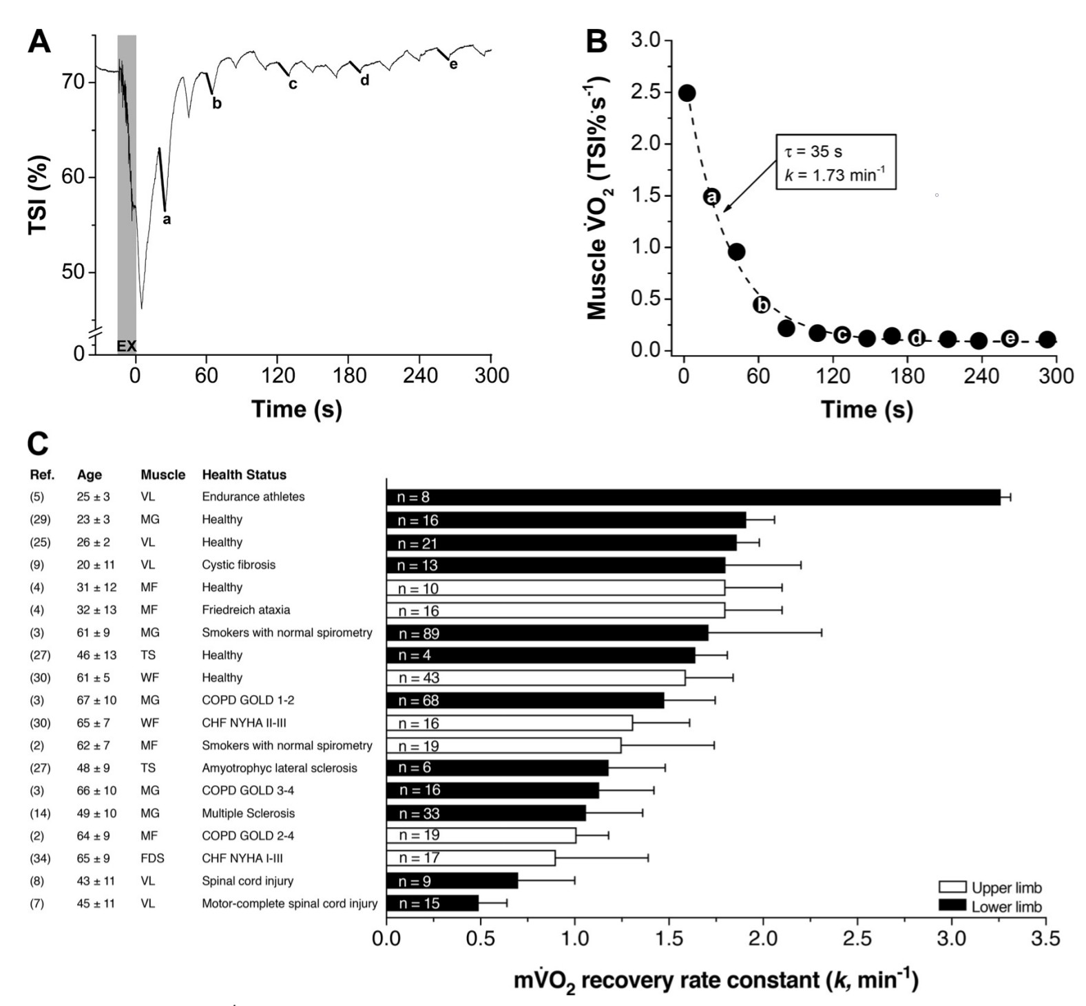
This technique has been well studied in recent years, validated against 31P-MRS [4] and mitochondrial content protein markers [5]. The rate constant k has been shown to be proportionally higher (faster recovery) in endurance-trained muscle, and lower (slower) in pathalogical and diseased muscle [3].
A call for standardised processing methods
Technical procedures and analysis methods for OxCap assessment have converged toward standardisation in recent years, with methods showing good reliability and reproducibility.
Recently there has been a call to implement standard analysis scripts with robust slope detection and non-linear modelling, to minimise operator-related variability between research centres, and thereby improving interpretation of outcomes across populations and interventions [6,7].
I wanted to see how well (or poorly) my current {mnirs} functionality could process and analyse repeated occlusion muscle OxCap data.
In the future, this process will be wrapped into convenience functions to make the process easier for the end user. But I believe this process is already considerably simpler and more robust than non-reproducible methods relying on manual data cleaning, occlusion interval selection, and curve fitting.
Oxidative capacity analysis in {mnirs}
This article serves as a vignette for three analysis functions recently added to the {mnirs} package, and how they can be used together to perform robust OxCap analysis.
extract_intervals(): is used to detect specific events or times in anmnirsdata frame, and extract an interval around each one, returning a list of data frames.
This is useful when a certain event is labelled inevent_channel, or a list of time values is provided manually for when events occur, such as the start of an exercise interval or occlusion. The returned list of data frames is ready for further analysis. See?extract_intervalsfor more details.peak_slope(): is used to find the peak positive or negative linear regression slope from a numeric vector and return the slope value, intercept, and associated parameters.
The segment of an mNIRS signal with the steepest slope is often interpreted to represent the point of greatest mismatch between O2 supply and O2 demand, such as for muscle OxCap testing. See?peak_slopefor more details.monoexponential(): specifies the equation for an exponential function. Two self-starting functions are available for non-linear curve fitting;SS_monoexp4()fits a 4-parameter monoexponential model, whileSS_monoexp3()fits a reduced 3-parameter model without a time delay parameter, where monoexponential response is expected to be instantaneous.
Calling these functions in non-linear curve fitting functions (e.g.nls()) will return model coefficients for the three or four parameters. See?monoexponentialand?SS_monoexpfor more details.
Analysis plan
For OxCap analysis, we will perform roughly 8 steps:
- Import an example NIRS file with the repeated occlusions procedure.
- Pre-process/clean data, as needed (minimal in this example).
- Iteratively correct NIRS values for changes in blood volume, a required step to ensure valid analysis.
- Specify occlusion events in the data and extract a 5-sec intervals for all occlusions.
- Find the peak 3-sec linear regression NIRS slope within each occlusion event.
- Model a monoexponential curve fit across NIRS slope observations within both repeated occlusion trials.
- Extract the rate constant (k) for each trial exponential curve.
- Plot the modelled data.
My aim is to perform this analysis using only the {mnirs} package and {tidyverse} functions, keeping the script as clean as possible, with as few janky manual adjustments as necessary.
Setup
First, load our packages and initial setup options. We will silence {mnirs} info messages and set our ggplot2 theme.
Note
I received this example file from Dr. Thomas Tripp, Postdoctoral fellow in Dr. Martin MacInnis’ lab at the University of Calgary. They have kindly allowed me to include this file with the {mnirs} package for users to examine themselves.
It can be accessed by calling
example_mnirs("portamon-oxcap").
This article will assume basic familiarity with the {mnirs} package. For further details and demonstration of data processing, please see the package vignette Reading and Cleaning Data with {mnirs}.
Read {mnirs} data file
The included example file has three NIRS channels and a column with sample number, which will automatically be converted to a time value when the read_mnirs() function recognises the Artinis Oxysoft export format and sample rate (10 Hz). The file does not need to be cleaned for outliers or digitally filtered, so minimal pre-processing is required.
One thing to note: Artinis Oxysoft exports an event label column without a named header by default. This is the column we will use to identify our occlusion events by the label "Occlusion", so we need to include it. Currently in {mnirs} an unnamed column like this will be named "col_" with a numeric suffix for the column number in the data file. In our example file, this events column will therefore be "col_6". It’s not the most elegant solution, but it works for now!
We can separate the two trials in the data set by finding the longer gap between consecutive occlusion labels and manually defining intervals before that as trial 1, and after that as trial 2.
df <- read_mnirs(
    file_path = example_mnirs("portamon-oxcap.xlsx"),
    nirs_channels = c(thb = 2, hhb = 3, o2hb = 4), ## identify and rename NIRS channels
    time_channel = c(sample = 1),
    event_channel = c(event = "col_6") ## specify the unnamed events column
)

## view the structure of our data frame
df
#> # A tibble: 7,944 × 6
#>    sample  time event   thb   hhb  o2hb
#>     <dbl> <dbl> <chr> <dbl> <dbl> <dbl>
#>  1      0   0   <NA>   146.  63.0  82.9
#>  2      1   0.1 <NA>   146.  63.0  82.8
#>  3      2   0.2 <NA>   146.  63.0  82.8
#>  4      3   0.3 <NA>   146.  63.0  82.9
#>  5      4   0.4 <NA>   146.  63.0  82.7
#>  6      5   0.5 <NA>   146.  62.9  82.6
#>  7      6   0.6 <NA>   146.  62.9  82.7
#>  8      7   0.7 <NA>   146.  62.9  82.8
#>  9      8   0.8 <NA>   146.  62.9  82.7
#> 10      9   0.9 <NA>   146.  62.9  82.7
#> # ℹ 7,934 more rows

## "Occlusion" is our pre-specified event string in our events column
## find each occlusion event, find where there is a longer gap
## the number of occlusions before this should be in the first trial
df_occlusions <- df[grepl("Occlusion", df$event), ]
n_occlusions <- which(diff(df_occlusions$time) > 60)

plot(df)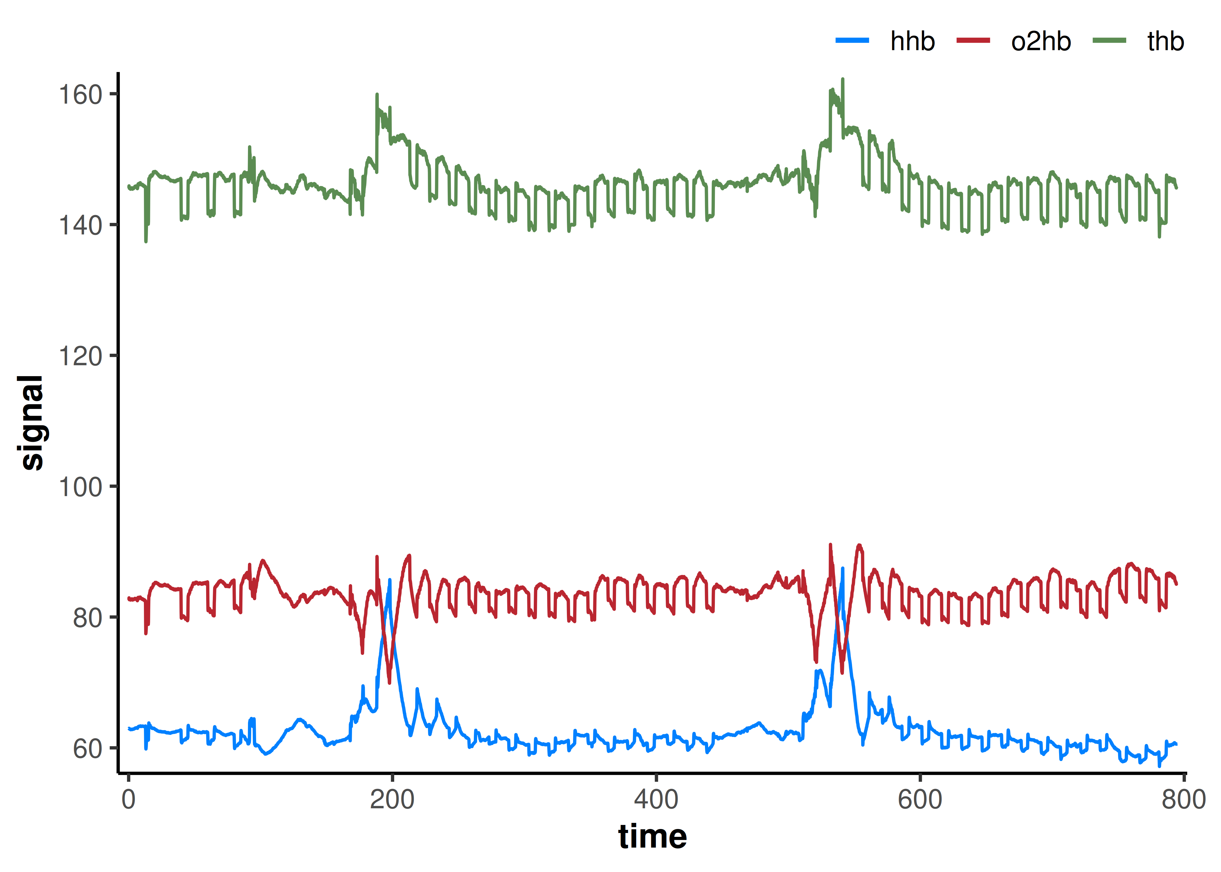
The two exercise bouts and repeated occlusion trials can clearly be identified from plotting the raw data. A few resting occlusions were also performed at the start of the file, but we will ignore those and just model the two repeated occlusion trials.
Correct for blood volume
A necessary processing step before analysing the OxCap trials is to apply a correction to the NIRS channels for changes in blood volume during the repeated occlusions. This step has been shown to improve validity when taking slopes of the oxy- or deoxyhaeme channels [8].
The preferred method is to iteratively correct for instantaneous changes in oxygenation between samples, according to Beever et al, 2020 [1].
df <- df |>
    mutate(
        ## blood volume correction factor beta, requires all positive values
        beta = o2hb / (o2hb + hhb),
        ## use {purrr} to iteratively adjust NIRS values from one sample to the next
        ## corrected for change in blood volume by beta since the previous sample
        o2hb = purrr::accumulate(2:n(), \(prev, i) {
            prev + (o2hb[i] - o2hb[i - 1]) - beta[i] * (thb[i] - thb[i - 1])
            }, .init = 0
        ),
        hhb = purrr::accumulate(2:n(), \(prev, i) {
            prev + (hhb[i] - hhb[i - 1]) - (1 - beta[i]) * (thb[i] - thb[i - 1])
            }, .init = 0
        ),
        ## thb corrected for changes in blood volume becomes equal to zero
        thb = o2hb + hhb,
    )

## plot corrected data with occlusion event indicators
plot(df) +
    geom_vline(xintercept = df_occlusions$time, linetype = "dotted", alpha = 0.4)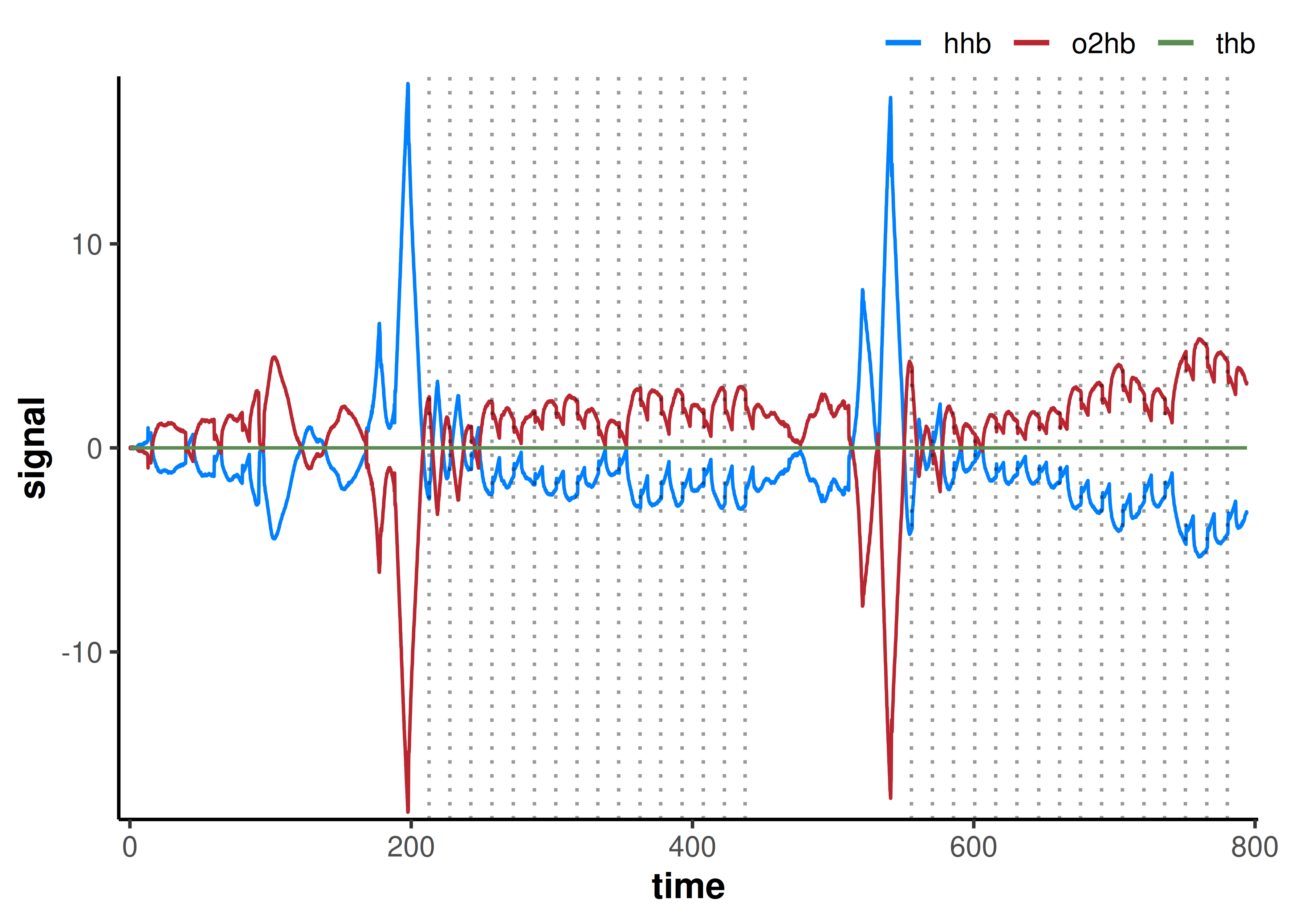
This results in a symmetrical distribution of oxy- and deoxyhaeme, with the sum total (total-haeme; THb) equal to zero at all samples.
We can also plot occlusion event indicators (vertical dotted lines) to confirm timing and detect any missed/extra events.
Extract occlusion intervals
The next step is to identify these occlusion events and extract the interval around each, into a list of data frames which we can continue to analyse iteratively.
extract_intervals()
-
dataThis function takes in a data frame, applies processing to all channels specified, then returns a list of processed data frames.
mnirsmetadata will be passed to and from this function.
For this analysis, we will re-join the returned list of data frames into a combined data frame with a grouping variable labelled “interval”. -
nirs_channels,time_channel,event_channel, &sample_rateSpecify which column names in
datawill be processed.nirs_channelsare the response variables;time_channelis the time series variable;event_channelspecifies where to look for event labels; andsample_ratespecifies the recording rate used when ensemble-averaging across intervals with unequal time samples. If any arguments are not specified, they will be retrieved frommnirsmetadata. Channels in the data but not explicitly specified will be passed through unprocessed to the returned data frames.
We will analyse OxCap from the deoxyhaeme (HHb) NIRS signal, which is often recommended [6]. -
event_times,event_labels, &event_samplesInterval events can be specified by any combination of time (values of
time_channel), labels (values ofevent_channel), or sample (row number). Multiple values can be entered as vectors. At least one event must be specified.
Once again, in this example data file, the occlusions are all identified by the event label"Occlusion". This makes it very simple to detect this string in theeventcolumn, and extract intervals around them.
Detecting intervals by event labels must match a full string exactly. If the event labels are inconsistent, we could specify a regular expression (regex) string such as"(?i)occlusions?"or"start|end". -
spanWhere an event is detected, an interval will be extracted with a time span specified as a two-element numeric vector;
c(start, end), in units of thetime_channel. Where positive values represent times after the event, and negative values represent times before the event.
All occlusion bouts were held for 5-seconds in this protocol. If the occlusion duration changed across the protocol, we might have to specify a list of time spans, rather than a singlespanas in this case.
From visual investigation of the plots, we were able to see that in the first ~0.5 sec after the occlusion label, the deoxyhaeme signal was disrupted by the inflation of the cuff, which might produce invalid slope values. So we will specify a time span ofc(1, 5), i.e. from 1 to 5 seconds after each"Occlusion"event label. If we wanted to include an interval before the event label, we could specify a negative numeric value, e.g.c(-2.5, 2.5)to include a 5-sec span centred on the label itself. -
group_eventsMultiple events can be extracted for analysis as
"distinct"intervals, or"ensemble"-averaged together. Different groupings of intervals can be ensemble-averaged by providing a list of numeric vectors specifying event intervals by number to ensemble-average or return as distinct; e.g.list(c(1, 2), c(3, 4)).
The interval numbers need to be known ahead of time and always refer to their order of occurrence in the data frame (i.e., sorted bytime_channel). Any event intervals detected but not supplied by number will be included as distinct data frames. -
zero_timeThe time values for each event interval can be recalculated to start from zero at the event indicator. Time values for ensemble-averaged intervals will always be re-calculated from zero, since the original time information is lost when ensembling.
For repeated occlusion testing, the original time information for each occlusion interval is critical to subsequently model the exponential recovery function, so we keep this asFALSE.
## identify and extract intervals by event label
## re-join the returned list of data frames with each occlusion interval labelled as "interval"
df_list <- extract_intervals(
    df,
    nirs_channels = hhb,        ## only required to specify nirs_channels when ensemble-averaging
    event_labels = "Occlusion", ## event label used in file, must match string exactly
    span = c(1, 5),             ## occlusion interval c(start, end) with reference to the event time value
    group_events = "distinct",  ## return each occlusion event separately
    zero_time = FALSE           ## preserve original time values at each event
) |>
    ## join back into a single grouped data frame, mostly for easier plotting below
    purrr::list_rbind(names_to = "interval") |>
    ## convert the "interval" column to a categorical factor
    mutate(interval = factor(interval, levels = unique(interval))) |>
    ## add `mnirs` metadata back to the combined data frame, for plotting
    create_mnirs_data(
        attributes(df)[c(
            "nirs_channels",
            "time_channel",
            "event_channel",
            "sample_rate"
        )]
    )

## visualise facet plot with all occlusion intervals for error checking
## the steepest facets will be the first occlusions from the two trials
plot(df_list) +
    theme(
        strip.text = element_blank(),
        strip.background = element_blank(),
        strip.placement = "outside",
        axis.text.x = element_blank(),
    ) +
    facet_wrap(~interval, scales = "free_x", nrow = 4)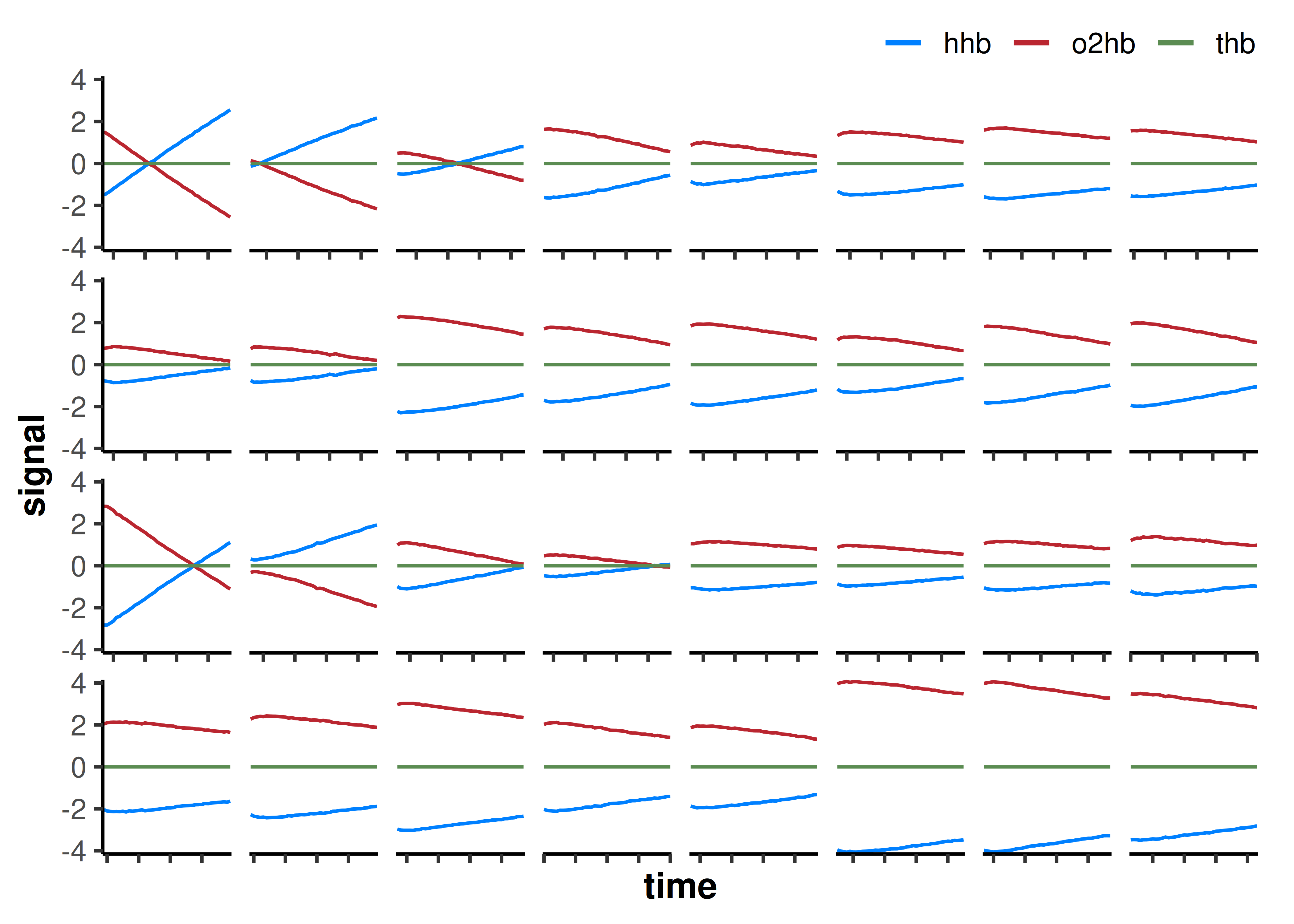
We can plot the sequence of extracted occlusion intervals to visually inspect the data. As expected, the first interval during each repeated occlusion trial appears the steepest, with the slope rapidly becoming less steep during each subsequent occlusion as mV̇O2 recovers.
From here, we want to calculate the slope values for each of these occlusion intervals.
Calculate occlusion slopes
peak_slope()
-
x,tThis function takes in a vector of numeric data (
x) and optional time values (t), processes the response variablexto find the peak local linear regression slope over the predictor variablet(defaults to sample number if not provided), and returns a list of parameters from that linear regression model. -
width,spanLinear regression is performed within a rolling local window specified by one of either
widthorspan.widthdefines a number of samples, whereasspandefines a range of time in units oftime_channel.
For this occlusion protocol, the peak 3-sec slope will be extracted from each 5-sec occlusion interval. -
alignThe local rolling linear regression window can be
"centre"-aligned around the target sample (idx), or it can be"left"-aligned withidxat the start of the window (forward-looking), or"right"-aligned withidxat the end of the window (backward-looking). -
directionBy default, the peak positive (upward) or negative (downward) slope will be returned depending on the overall trend direction of the response variable
x. This can be overridden by specifying either"positive"or"negative".
For processing deoxyhaeme, we will specify that the peak slope during occlusion should be positive, because deoxygenation increases. -
partialBy default, a local window will only return a linear regression model if all samples within the window are valid. If
partialis set toTRUE, then local windows will return a slope model as long as there are two or more valid samples.
A window with fewer samples will tend to return steeper slope values, which may or may not be relevant to our interpretations. e.g., as an edge-case (literally at the edges of the data) in a noisy data set there may be two samples with an extreme local slope between them. We usually would want to ignore this outlier slope value.
## iteratively find peak local slopes within each occlusion interval
## return summary values for each factor level of "interval" grouping column
slopes_df <- df_list |>
    reframe(
        .by = interval,
        {
            slope_params <- peak_slope(
                x = hhb, ## response variable: deoxyhaeme
                t = time, ## predictor variable: time in seconds
                span = 3, ## steepest 3 sec slope
                align = "left", ## forward-looking from index sample
                direction = "positive", ## upward slope for hhb
                partial = FALSE ## allow only complete 3-sec segments, no NAs
            )
            ## return time value (start time of 3-sec period) and slope value (μM/sec)
            data.frame(
                time = slope_params$t,
                slope = slope_params$slope
            )
        }
    ) |>
    mutate(
        ## manual factor by occlusions in each trial
        trial = factor(if_else(row_number() %in% seq_len(n_occlusions), 1L, 2L))
    ) |>
    mutate(
        ## recalculate time as starting from zero for each trial
        .by = trial,
        time = time - time[1L],
    ) |>
    select(trial, time, slope)

## create plot template
p <- ggplot(slopes_df, aes(time, slope, colour = trial)) +
    coord_cartesian(ylim = c(0, NA)) +
    scale_x_continuous(
        name = "Time (mm:ss)",
        breaks = breaks_timespan(),
        labels = format_hmmss
    ) +
    scale_y_continuous(expand = expansion(c(0, 0.03))) +
    scale_colour_mnirs() +
    labs(
        y = expression(bold(HHb ~ Slope ~ '(μM' %.% sec^'-1' * ')'))
    )

## plot observed slope values for each trial
p +
    geom_line() +
    geom_point(fill = "white", size = 3, shape = 21, stroke = 1)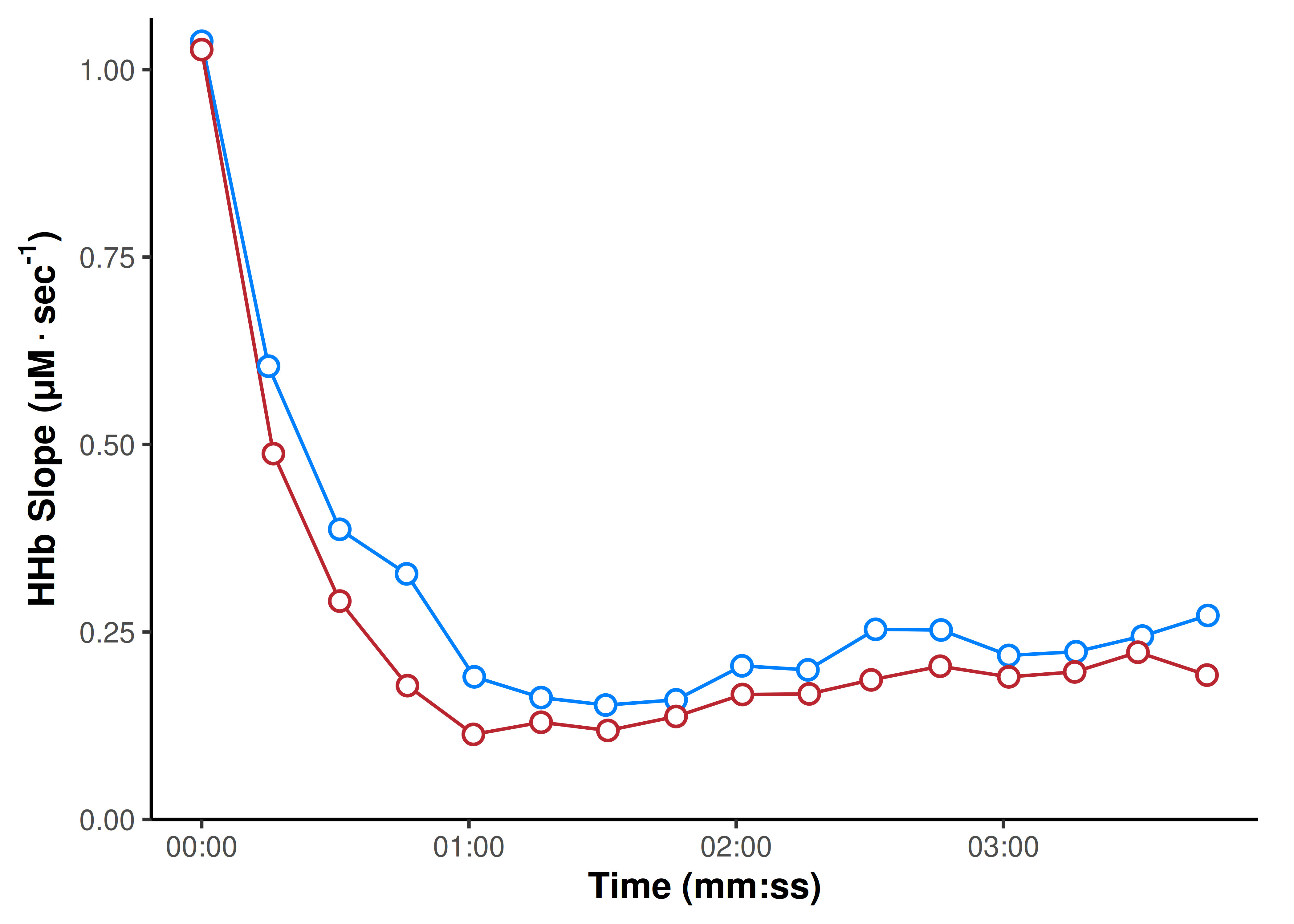
Plotting the returned slope values gives us a very nice indication of the exponential recovery response for mV̇O2 after each brief exercise task.
Model mV̇O2 recovery
monoexponential()
-
tThis function is the equation for either a 3- or 4-parameter monoexponential function. It takes in a predictor variable for time (
t) and generates the response variable (y) for an exponential curve with characteristics determined by four coefficients. -
A,BThe starting (baseline) value and the ending (asymptote) value, respectively for the monoexponential curve. Will define either an exponential association curve in the positive direction when
B>A, or exponential decay in the negative direction whenA>B. -
tauThe time constant (𝜏) of the exponential function determines the steepness of the initial slope of the curve. Tau is approximated by the time required to converge 63.2% of the amplitude between
AandB.
The rate constant (k) is the inverse of the time constant (k = 1 / tau) and is also commonly used in NIRS research, including for OxCap assessment. In this example we will report k in units of min-1. -
TDTD is the optional fourth parameter which defines a time lag before the start of monoexponential behaviour. This can capture behaviour which does not respond instantaneously to an intervention with a delay or a transient acceleration phase before exponential behaviour.
Often during repeated occlusions after exercise, the first occlusions may not conform to monoexponential behaviour, if the oxygen saturation is too low and limiting to mV̇O2. In these cases, a time delay parameter may be required to accurately capture the true monoexponential response. This example protocol was designed to avoid this potential delay and so a time delay parameter was not required.
SS_monoexp3(), SS_monoexp4()
- These self-starting non-linear curve functions allow for optimising monoexponential fit coefficients on existing data, with either a 3- or 4-parameter model using
nls()or another non-linear optimiser function. They return a model with three or four coefficients and associated fit parameters.
Having split our data set of times and slopes by trial, we can use tidyr::nest() purrr::map() functions to iteratively fit a 3-parameter monoexponential model for slope over time, for each trial, and return the primary outcome coefficient; the rate constant (k), calculated as the inverse of the time constant (tau).
## use 3-param monoexponential model for each trial
## return fitted curve and time constant tau coefficient
pred_df <- slopes_df |>
    ## nest the data to model each trial
    tidyr::nest(.by = trial) |>
    mutate(
        ## apply self-starting monoexp model to each trial
        model = purrr::map(data, \(.df) {
            nls(slope ~ SS_monoexp3(time, A, B, tau), data = .df)
        }),
        ## return tau coefficient for each trial model
        tau = purrr::map_dbl(model, \(.m) coef(.m)[["tau"]]),
        ## return the predicted exponential curve values for plotting
        data = purrr::map2(data, model, \(.df, .m) {
            mutate(.df, predicted_slope = predict(.m))
        })
    ) |>
    select(trial, tau, data) |>
    ## unnest back into the top level data frame for extraction and plotting
    tidyr::unnest(data)

## extract tau and k coef labels per trial, for plotting
coef_df <- pred_df |>
    summarise(
        .by = trial,
        label = stringr::str_glue(
            "Trial {trial[1]}
            tau = {mnirs:::signif_trailing(tau[1], 1)} sec
            k = {mnirs:::signif_trailing(60 / tau[1], 1)} min⁻¹"
        )
    )
## add predicted values to the plot of observed data
p +
    geom_line(
        data = pred_df,
        aes(y = predicted_slope, group = trial),
        colour = "black", linewidth = 1
    ) +
    geom_text(
        data = coef_df,
        aes(label = label, colour = trial, group = trial),
        x = Inf, y = Inf,
        size = 5, hjust = 1.1, vjust = c(1.5, 3)
    ) +
    geom_line() +
    geom_point(fill = "white", size = 3, shape = 21, stroke = 1)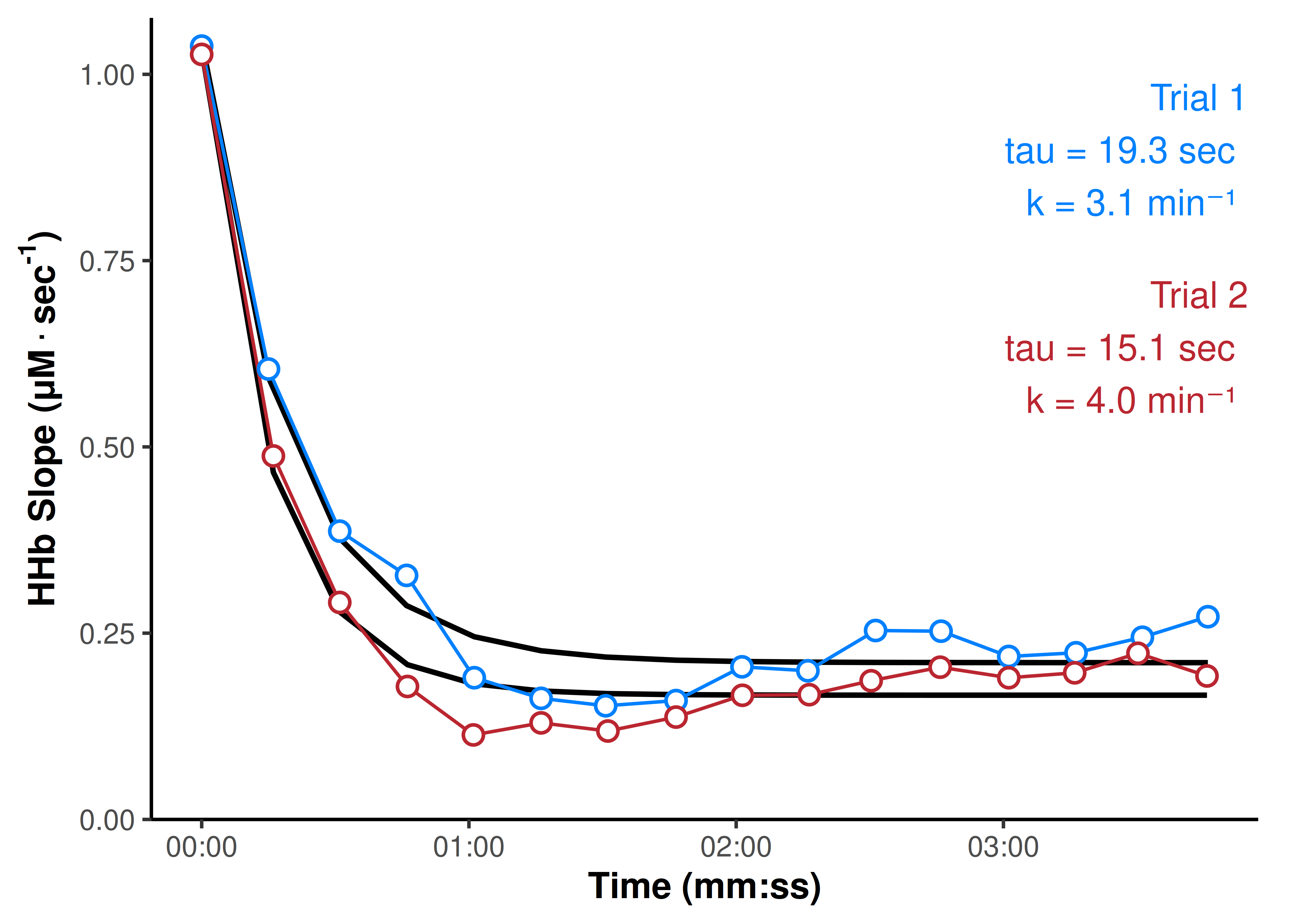
Conclusion
This article demonstrates how muscle oxidative capacity analysis can be performed using {mnirs} and some relatively simple, reproducible data wrangling steps.
In future development, I would like to wrap some of these processing steps into dedicated functions with recommended default parameters, to make the analysis process more streamlined.
However, there are also a few limitations to this current process: modelling monoexponential behaviour with relatively few data samples (there are 17 occlusions per trial in this example) can result in unstable fit parameters or inability to converge non-linear fitting at all.
A more robust fitting process may be required for real-world data where mV̇O2 recovery does not perfectly conform to monoexponential behaviour. Or, manual processing steps may be inevitably required during analysis to accommodate for these computational limitations.