Biexponential function

Calculate a two-phase curve: a fast monoexponential primary response toward B and a slow monoexponential secondary response from B toward a stable plateau at B2, both clocked from the response onset and summed. Model family fit by analyse_kinetics() with method = "biexponential", and by stats::nls() via the self-starting wrapper SSbiexponential().

Usage

biexponential(t, A, B, tau, B2, tau2, TD = NULL)

Arguments

t: A numeric vector of the predictor variable (time).
A: A numeric parameter for the starting value of the response variable (the t = 0 intercept).
B: A numeric parameter for the asymptote of the fast component; the value the fast response alone would approach.
tau: A numeric parameter for the fast time constant (\(\tau_1\)), in units of the predictor variable t. Dominates the initial steep response.
B2: A numeric parameter for the asymptote of the slow component; the stable plateau the response recovers toward as t approaches infinity.
tau2: A numeric parameter for the slow time constant (\(\tau_2\)), in units of the predictor variable t. Typically tau2 >> tau.
TD: A numeric parameter for the time delay before the onset of the response, in units of the predictor variable t. If NULL (default), a 5-parameter model without time delay is used.

Value

A numeric vector of predicted values the same length as the predictor variable t.

Details

Model equations

5-parameter: A + (B - A) * (1 - exp(-t / tau)) + (B2 - B) * (1 - exp(-t / tau2))
6-parameter, where ts = pmax(t - TD, 0): A + (B - A) * (1 - exp(-ts / tau)) + (B2 - B) * (1 - exp(-ts / tau2))

A, B, and B2 are all values on the response scale. The fast component is a monoexponential() response from A toward B with amplitude B - A; the slow component runs concurrently from the same onset with amplitude B2 - B. The curve starts at A, approaches B2 as t grows, and is smooth throughout. If B = B2, the curve reduces to a monoexponential() with time constant tau and asymptote B2.

Excursion point

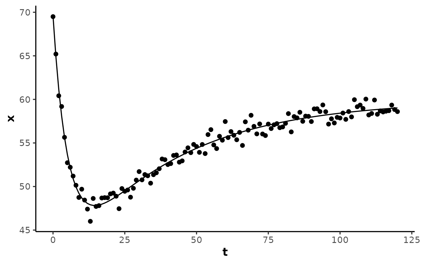
The expected response is a fast excursion toward a minimum or maximum short of B, followed by a slow recovery back to a stable plateau at B2. The excursion point texc occurs where the two phase rates cancel: texc = TD + log(ratio) / (1 / tau - 1 / tau2) with ratio = -(B - A) * tau2 / ((B2 - B) * tau), which exists only when the amplitudes oppose in sign and the fast phase dominates at the onset (ratio > 1). If B is between A and B2, the response is monotonic but still two-phase.

Examples

## create a biexponential excursion-recovery curve with random noise
set.seed(1)
t <- 0:120
x <- biexponential(t, A = 70, B = 40, tau = 5, B2 = 60, tau2 = 40) +
    rnorm(length(t), 0, 0.8)
data <- data.frame(t, x)

## 5-parameter fit with the self-starting wrapper
model <- nls(
    x ~ SSbiexponential(t, A, B, tau, B2, tau2),
    data = data,
    algorithm = "port",
    lower = c(-Inf, -Inf, 0, -Inf, 0),
    control = nls.control(warnOnly = TRUE)
)
summary(model)
#> 
#> Formula: x ~ SSbiexponential(t, A, B, tau, B2, tau2)
#> 
#> Parameters:
#>      Estimate Std. Error t value Pr(>|t|)    
#> A     69.5786     0.5490  126.73   <2e-16 ***
#> B     39.2594     1.1326   34.66   <2e-16 ***
#> tau    5.3301     0.3158   16.88   <2e-16 ***
#> B2    59.8830     0.3273  182.97   <2e-16 ***
#> tau2  37.8230     3.0486   12.41   <2e-16 ***
#> ---
#> Signif. codes:  0 ‘***’ 0.001 ‘**’ 0.01 ‘*’ 0.05 ‘.’ 0.1 ‘ ’ 1
#> 
#> Residual standard error: 0.7114 on 116 degrees of freedom
#> 
#> Algorithm "port", convergence message: relative convergence (4)
#> 

y <- predict(model, data)

# \donttest{
    if (requireNamespace("ggplot2", quietly = TRUE)) {
        ggplot2::ggplot(data, ggplot2::aes(t, x)) +
            theme_mnirs() +
            ggplot2::geom_point() +
            ggplot2::geom_line(ggplot2::aes(y = y))
    }

# }