Fractional response time

Estimate the time at which a numeric vector reaches a specified fraction of its total response amplitude relative to a baseline, e.g. half-response time at response_fraction = 0.5. Vector-level companion to analyse_kinetics() with method = "response_time".

Usage

response_time(
  x,
  t = seq_along(x),
  start_time = 0,
  response_fraction = 0.5,
  direction = c("auto", "positive", "negative"),
  verbose = TRUE,
  ...
)

Arguments

x

A numeric vector of the response variable.

t

An optional numeric vector of the predictor variable (e.g. time). Default is seq_along(x).

start_time

A numeric value in units of t specifying the response onset. Samples where t <= start_time define the baseline window. Default is 0.

response_fraction

A numeric vector in the range [0, 1] specifying the fractional response amplitude(s) to detect. Defaults to 0.5 (50% response, i.e. half-response time). Multiple values (e.g. c(0.5, 0.632)) return one element per fraction.

direction

A character string specifying the response direction "positive", or "negative", or detect with "auto" (default). See Details.

verbose

Logical. TRUE (default) will display, and FALSE will silence warnings and information messages helpful for troubleshooting. Global default can be set via options(mnirs.verbose = FALSE).

...

Additional arguments.

Value

A named list containing:

A

The mean baseline value of x where t <= start_time.

B

The extreme (maximum or minimum) value of x after start_time.

response_time

The elapsed time from start_time to the fractional response, in units of t; one element per response_fraction.

response_value

The observed value of x at the response index; one element per response_fraction.

fitted

The target fractional response value A + (B - A) * response_fraction; one element per response_fraction.

baseline_idx

Integer indices where t <= start_time.

response_idx

Integer index at each response_value.

extreme_idx

Integer index at the extreme value B.

Details

A non-parametric approach (estimated directly from the observed data without assuming a specific mathematical shape). response_fraction = 0.5 approximates the inflection point (xmid) of a symmetric sigmoid function. response_fraction = 0.632 approximates the time constant (tau; \(\tau\)) of a monoexponential function, or xmid of a left-Gompertz function. response_fraction = 0.368 approximates xmid of a right-Gompertz function. This is a good fallback estimation method if parametric methods are not successfully fit.

Method

The target response value is: fitted = A + (B - A) * response_fraction

Where A is the mean baseline value (t <= start_time) and B is the extreme (peak or trough) value after start_time. response_value is the first observed sample equal to or greater/lesser than the target fitted value (above for "positive", below for "negative" direction). response_time is the elapsed time from start_time to response_value.

analyse_kinetics() first trims x to end_window past the first extreme, so B there is the first local extreme with no greater/lesser values within end_window. Called directly, B is the global extreme of x after start_time.

Direction

direction is detected automatically by default as either "positive" (upward) or "negative" (downward) response, from the dominant excursion of x above or below its initial baseline (the median of the earliest samples). When tied, the greater absolute extreme decides. B is the maximum for "positive" or the minimum for "negative", and can be overwritten manually.

Baseline

When no samples exist where t <= start_time, the first sample x[1] is used as the baseline A with a warning. start_time must be within the range of t.

See also

analyse_kinetics(), peak_slope(), monoexponential()

Examples

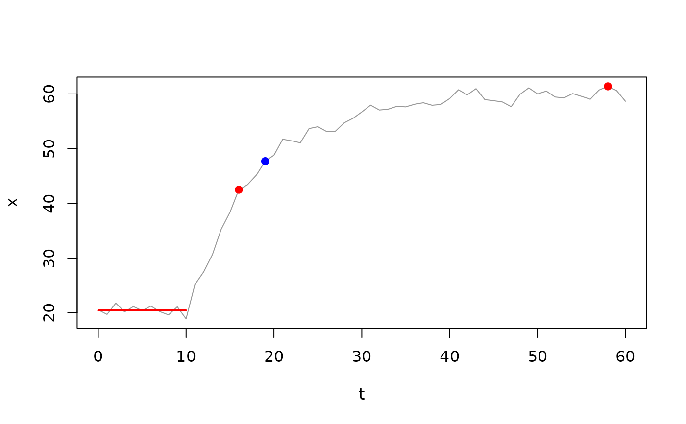
## create an exponential curve with random noise
set.seed(13)
t <- 0:60
x <- monoexponential(t, A = 20, B = 60, tau = 8, TD = 10) +
    rnorm(length(t), 0, 1)

## half-response time (0.5) and time constant approximation (0.632 ~= tau)
RT <- response_time(x, t, start_time = 10, response_fraction = c(0.5, 0.632))
RT$response_time
#> [1] 6 9

plot(t, x, type = "l", col = "grey60", xlab = "t", ylab = "x")
## mean baseline `A` across the baseline window
segments(
    t[min(RT$baseline_idx)], RT$A,
    t[max(RT$baseline_idx)], RT$A,
    col = "red", lwd = 2
)
## response values at 0.5 (red) and 0.632 (blue), and the extreme `B`
points(
    t[RT$response_idx],
    RT$response_value,
    col = c("red", "blue"),
    pch = 19
)
points(t[RT$extreme_idx], RT$B, col = "red", pch = 19)