
{mnirs} contains standardised, reproducible methods for reading, processing, and analysing data from muscle near-infrared spectroscopy (mNIRS) devices. Intended for mNIRS researchers and practitioners in exercise physiology, sports science, and clinical rehabilitation with minimal coding experience required.
Installation
install.packages("mnirs")You can install the development version of mnirs from GitHub with:
# install.packages("pak")
pak::pak("jemarnold/mnirs")Online App
A very basic implementation of this package is hosted at https://jemarnold-mnirs-app.share.connect.posit.cloud/ and can currently be used for reading and pre-processing mNIRS data.
Usage
A more detailed vignette for common usage can be found on the package website: Reading and Cleaning Data with {mnirs}
mnirs is designed for mNIRS data, but it can be used to read, clean, and process other time series datasets which require many of the same processing steps. Enjoy!
read_mnirs() Read data from file
library(ggplot2) ## for plotting
library(mnirs)
## {mnirs} includes sample files from a few mNIRS devices
example_mnirs()
#> [1] "artinis_intervals.xlsx" "moxy_intervals.csv"
#> [3] "moxy_ramp.xlsx" "portamon-oxcap.xlsx"
#> [5] "train.red_intervals.csv"
## rename channels in the format `renamed = "original_name"`
## where "original_name1" should match the file column name exactly
data_raw <- read_mnirs(
file_path = example_mnirs("moxy_ramp"), ## call an example data file
nirs_channels = c(
smo2_left = "SmO2 Live", ## identify and rename channels
smo2_right = "SmO2 Live(2)"
),
time_channel = c(time = "hh:mm:ss"), ## date-time format will be converted to numeric
event_channel = NULL, ## leave blank if unused
sample_rate = NULL, ## if blank, will be estimated from time_channel
add_timestamp = FALSE, ## omit a date-time timestamp column
zero_time = TRUE, ## recalculate time values from zero
keep_all = FALSE, ## return only the specified data channels
verbose = TRUE ## show warnings & messages
)
#> ! Estimated `sample_rate` = 2 Hz.
#> ℹ Define `sample_rate` explicitly to override.
#> Warning: ! Duplicate or irregular `time_channel` samples detected.
#> ℹ `time` = 211.59 and 1183.6.
#> ℹ Re-sample with `mnirs::resample_mnirs()`.
## Note the above info message that sample_rate was estimated correctly at 2 Hz 👆
## ignore the warnings about irregular sampling for now, we will resample later
data_raw
#> # A tibble: 2,202 × 3
#> time smo2_left smo2_right
#> <dbl> <dbl> <dbl>
#> 1 0 54 68
#> 2 0.560 54 68
#> 3 1.11 54 66
#> 4 1.66 54 66
#> 5 2.21 54 66
#> 6 2.76 54 66
#> 7 3.31 57 67
#> 8 3.86 57 67
#> 9 4.41 57 67
#> 10 4.96 57 67
#> # ℹ 2,192 more rows
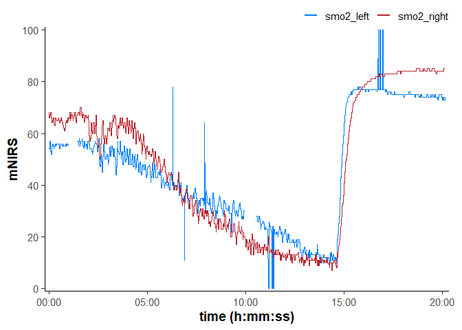
## note the `time_labels` plot argument to display time values as `h:mm:ss`
plot(
data_raw,
time_labels = TRUE,
na.omit = FALSE
)
resample_mnirs(): Resample data
data_resampled <- resample_mnirs(
    data_raw,            ## blank channels will be retrieved from metadata
    time_channel = time, ## channels can be left blank or specified explicitly
    sample_rate = NULL,  ## blank by default will be retrieved from metadata
    resample_rate = 2,   ## blank by default will resample to `sample_rate`
    method = "linear"    ## linear interpolation across resampled indices
)
#> ℹ Output is resampled at 2 Hz.

## note the altered "time" values from the original data frame 👇
data_resampled
#> # A tibble: 2,419 × 3
#>     time smo2_left smo2_right
#>    <dbl>     <dbl>      <dbl>
#>  1   0        54         68
#>  2   0.5      54         68
#>  3   1        54         66.4
#>  4   1.5      54         66
#>  5   2        54         66
#>  6   2.5      54         66
#>  7   3        55.3       66.4
#>  8   3.5      57         67
#>  9   4        57         67
#> 10   4.5      57         67
#> # ℹ 2,409 more rows
replace_mnirs: Replace local outliers, invalid values, and missing values
data_cleaned <- replace_mnirs(
    data_resampled,     ## blank channels will be retrieved from metadata
    invalid_values = 0, ## known invalid values in the data
    invalid_above = 90, ## remove data spikes above 90
    outlier_cutoff = 3, ## recommended default value
    width = 7,          ## window to detect and replace outliers/missing values
    method = "linear"   ## linear interpolation over `NA`s
)

plot(data_cleaned, time_labels = TRUE)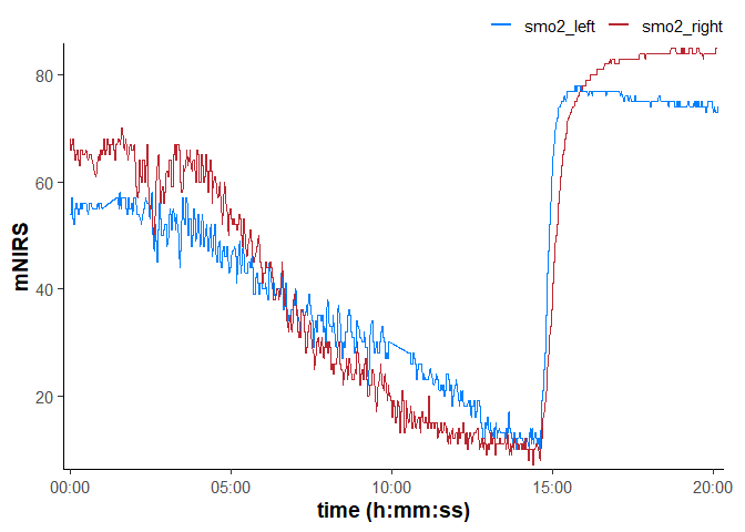
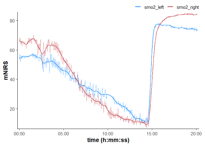
filter_mnirs(): Digital filtering
data_filtered <- filter_mnirs(
    data_cleaned,           ## blank channels will be retrieved from metadata
    method = "butterworth", ## Butterworth digital filter is a common choice
    order = 2,              ## filter order number
    W = 0.02,               ## filter fractional critical frequency `[0, 1]`
    type = "low",           ## specify a "low-pass" filter
    na.rm = TRUE            ## explicitly ignore NAs
)

## we will add the non-filtered data back to the plot to compare
plot(data_filtered, time_labels = TRUE) +
    geom_line(
        data = data_cleaned,
        aes(y = smo2_left, colour = "smo2_left"), alpha = 0.4
    ) +
    geom_line(
        data = data_cleaned,
        aes(y = smo2_right, colour = "smo2_right"), alpha = 0.4
    )
shift_mnirs() & rescale_mnirs(): Shift and rescale data
data_shifted <- shift_mnirs(
    data_filtered,     ## un-grouped nirs channels to shift separately
    nirs_channels = list(smo2_left, smo2_right),
    to = 0,            ## NIRS values will be shifted to zero
    span = 120,        ## shift the *first* 120 sec of data to zero
    position = "first"
)

plot(data_shifted, time_labels = TRUE) +
    geom_hline(yintercept = 0, linetype = "dotted")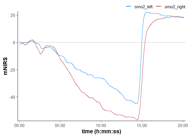
data_rescaled <- rescale_mnirs(
    data_filtered,    ## un-grouped nirs channels to rescale separately
    nirs_channels = list(smo2_left, smo2_right),
    range = c(0, 100) ## rescale to a 0-100% functional exercise range
)

plot(data_rescaled, time_labels = TRUE) +
    geom_hline(yintercept = c(0, 100), linetype = "dotted")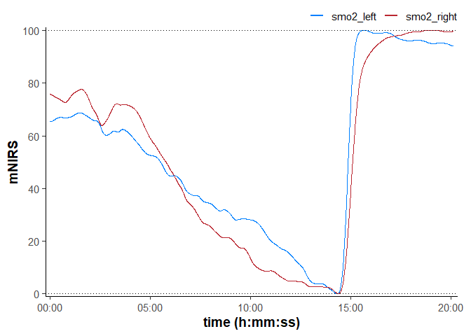
Pipe-friendly functions
## global option to silence info & warning messages
options(mnirs.verbose = FALSE)

nirs_data <- read_mnirs(
    example_mnirs("train.red"),
    nirs_channels = c(
        smo2_left = "SmO2 unfiltered",
        smo2_right = "SmO2 unfiltered"
    ),
    time_channel = c(time = "Timestamp (seconds passed)"),
    zero_time = TRUE
) |>
    resample_mnirs(method = "linear") |> ## default settings will resample to the same `sample_rate`
    replace_mnirs(
        invalid_above = 73,
        outlier_cutoff = 3,
        span = 7
    ) |>
    filter_mnirs(
        method = "butterworth",
        order = 2,
        W = 0.02,
        na.rm = TRUE
    ) |>
    shift_mnirs(
        nirs_channels = list(smo2_left, smo2_right), ## 👈 channels grouped separately
        to = 0,
        span = 60,
        position = "first"
    ) |>
    rescale_mnirs(
        nirs_channels = list(c(smo2_left, smo2_right)), ## 👈 channels grouped together
        range = c(0, 100)
    )

plot(nirs_data, time_labels = TRUE)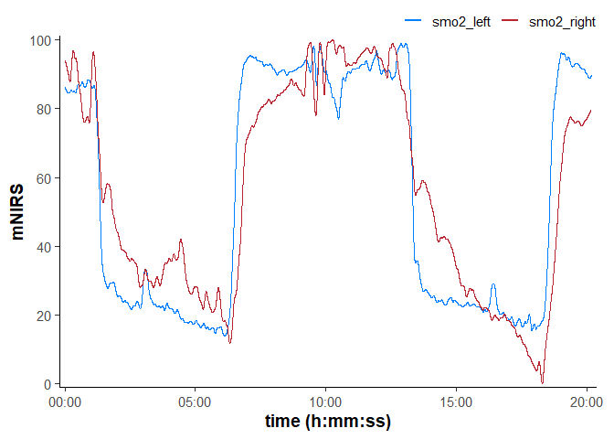
extract_intervals(): detect events and extract intervals
## return each interval independently with `event_groups = "distinct"`
distinct <- extract_intervals(
    nirs_data,                  ## channels blank for "distinct" grouping
    start = by_time(348, 1064), ## manually identified interval start times
    end = by_time(458, 1174),   ## interval end time (start + 150 sec)
    event_groups = "distinct",  ## return a list of data frames for each (2) event
    span = c(0, 0),             ## no boundary modification
    zero_time = FALSE           ## return original time values
)

plot(distinct, time_labels = TRUE)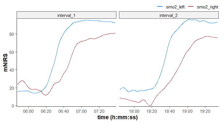
## ensemble average both intervals with `event_groups = "ensemble"`
ensemble <- extract_intervals(
    nirs_data,                  ## channels recycled to all intervals by default
    nirs_channels = c(smo2_left, smo2_right),
    start = by_time(368, 1084), ## alternatively specify start times + span
    event_groups = "ensemble",  ## ensemble-average across two intervals
    span = c(-20, 90),          ## span recycled to all intervals by default
    zero_time = TRUE            ## re-calculate common time to start from `0`
)

plot(ensemble, time_labels = TRUE) +
    geom_vline(xintercept = 0, linetype = "dotted")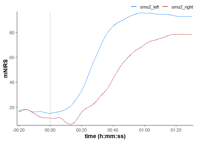
Future mnirs development
-
Process oxygenation kinetics
Monoexponential & sigmoidal non-linear curve fitting
Non-parametric response time & slope analysis
-
Critical oxygenation breakpoint analysis
- Manual selection and automation-assisted breakpoint detection (combine expert evaluation with robust probabilistic breakpoint detection)
-
Oxidative capacity assessment
Repeated occlusion ensemble-averaging and model fitting
Blood volume correction
mNIRS device compatibility
This package is designed to recognise mNIRS data exported as .csv or .xls(x) files. It should be flexible for use with many different NIRS devices, and compatibility will improve with continued development.
Currently, it has been tested successfully with mNIRS data exported from the following devices and apps:
- Artinis Oxysoft software (.csv and .xlsx)
- Moxy direct export (.csv)
- PerfPro PC software (.xlsx)
- Train.Red app (.csv)
- VO2 Master Manager app (.xlsx)
Generative chatbots are used to assist with code optimisation. All code is thoroughly reviewed and validated by the package author.