Exponential-drift function

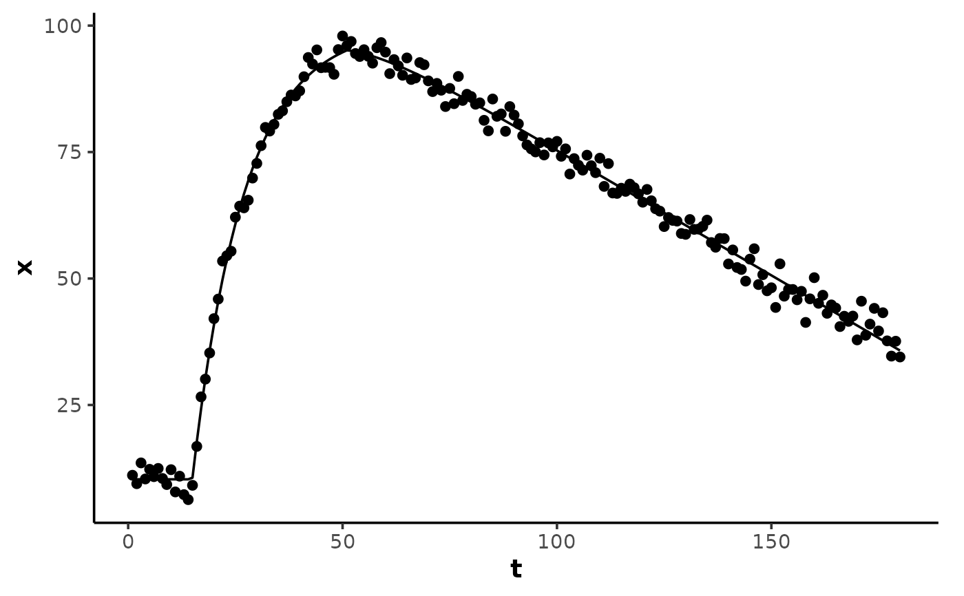
Calculate a two-phase curve: a fast monoexponential() primary response plus a slow linear secondary drift beginning near the primary asymptote. Model family fit by analyse_kinetics() with method = "exponential_drift", and by stats::nls() via the self-starting wrapper SSexponential_drift().

Usage

exponential_drift(t, A, B, tau, slope_B, drift_fraction, TD = NULL)

Arguments

t

A numeric vector of the predictor variable (time).

A

A numeric parameter for the starting baseline of the response variable.

B

A numeric parameter for the ending asymptote of the response variable.

tau

A numeric parameter for the time constant (\(\tau\)) of the exponential response, in units of the predictor variable t.

slope_B

A numeric parameter for the linear drift rate dx/dt of the secondary phase, in response units per unit of the predictor variable t.

drift_fraction

A numeric fraction of the primary amplitude B - A in (0.5, 1) at which the linear drift begins, where the primary response reaches A + drift_fraction * (B - A).

TD

A numeric parameter for the time delay before the onset of the exponential response, in units of the predictor variable t. If NULL (default), a 3-parameter model without time delay is used.

Value

A numeric vector of predicted values the same length as the predictor variable t.

Details

Model equations

• 5-parameter: A + (B - A) * (1 - exp(-t / tau)) + slope_B * pmax(t + tau * log(1 - drift_fraction), 0)

• 6-parameter: A + (B - A) * (1 - exp(-pmax(t - TD, 0) / tau)) + slope_B * pmax(t - TD + tau * log(1 - drift_fraction), 0)

A, B, tau, and TD are as for monoexponential(). The drift onset is not a free estimate: the secondary drift is exactly zero before TD - tau * log(1 - drift_fraction) (TD = 0 when absent), and drift_fraction = 0.95 places the onset at TD + 3 * tau.

The excursion point texc is where the drift rate overtakes the decaying primary rate, TD + tau * log(|B - A| / (|slope_B| * tau)), floored at the drift onset.

See also

analyse_kinetics(), SSexponential_drift(), monoexponential(), biexponential(), sigmoidal_drift()

Examples

## create an exponential curve with late linear drift and random noise
set.seed(13)
t <- 1:180
x <- exponential_drift(
    t, A = 10, B = 100, tau = 12,
    slope_B = -0.5, drift_fraction = 0.95, TD = 15
) + rnorm(length(t), 0, 2)
data <- data.frame(t, x)

## the drift onset fraction is held constant in the formula
model <- nls(
    x ~ SSexponential_drift(
        t, A, B, tau, slope_B, drift_fraction = 0.95, TD
    ),
    data = data,
    algorithm = "port",
    lower = c(-Inf, -Inf, 0, -Inf, 0),
    control = nls.control(warnOnly = TRUE)
)
summary(model)
#> 
#> Formula: x ~ SSexponential_drift(t, A, B, tau, slope_B, drift_fraction = 0.95, 
#>     TD)
#> 
#> Parameters:
#>          Estimate Std. Error t value Pr(>|t|)    
#> A       10.305631   0.558620   18.45   <2e-16 ***
#> B       99.612728   0.302186  329.64   <2e-16 ***
#> tau     12.062878   0.202335   59.62   <2e-16 ***
#> slope_B -0.495293   0.005346  -92.64   <2e-16 ***
#> TD      14.956965   0.167821   89.12   <2e-16 ***
#> ---
#> Signif. codes:  0 ‘***’ 0.001 ‘**’ 0.01 ‘*’ 0.05 ‘.’ 0.1 ‘ ’ 1
#> 
#> Residual standard error: 2.091 on 175 degrees of freedom
#> 
#> Algorithm "port", convergence message: relative convergence (4)
#> 

y <- predict(model, data)

# \donttest{
    if (requireNamespace("ggplot2", quietly = TRUE)) {
        ggplot2::ggplot(data, ggplot2::aes(t, x)) +
            theme_mnirs() +
            ggplot2::geom_point() +
            ggplot2::geom_line(ggplot2::aes(y = y))
    }

# }