Gompertz growth functions

Calculate 4-parameter Gompertz (asymmetric sigmoidal) curves. Model families fit by analyse_kinetics() with method = "sigmoidal" and shape = "gompertz" or "gompertz_left", and by stats::nls() via the self-starting wrappers SSgompertz() and SSgompertz_left().

Usage

gompertz(t, A, B, xmid, slope)

gompertz_left(t, A, B, xmid, slope)

Arguments

t: A numeric vector of the predictor variable (time).
A: A numeric parameter for the starting asymptote of the response variable.
B: A numeric parameter for the ending asymptote of the response variable.
xmid: A numeric parameter for the time at the inflection point (the steepest point) of the curve, in units of the predictor variable t.
slope: A numeric parameter for the response rate dx/dt at the inflection xmid.

Value

A numeric vector of predicted values the same length as the predictor variable t.

Details

gompertz() (right-Gompertz) is asymmetric with the inflection point xmid closer to the starting asymptote A: early acceleration away from A, and a slow approach to the ending asymptote B. Appropriate for fast-onset, slow-tail responses.

gompertz_left() (left-Gompertz) has the inflection point closer to the ending asymptote B: slow departure from A, and late acceleration toward B. Appropriate for slow-onset, fast-tail responses.

Model equations

Both forms are re-parameterised so xmid is the time at inflection and slope is the response rate dx/dt at the inflection, with k = slope * e / (B - A).

gompertz(): A + (B - A) * exp(-exp(-k * (t - xmid))). Inflection height fixed at A + (B - A) / e; 36.8% of the amplitude.
gompertz_left(): A + (B - A) * (1 - exp(-exp(k * (t - xmid)))). Inflection height fixed at A + (B - A) * (1 - 1/e); 63.2% of the amplitude.

Examples

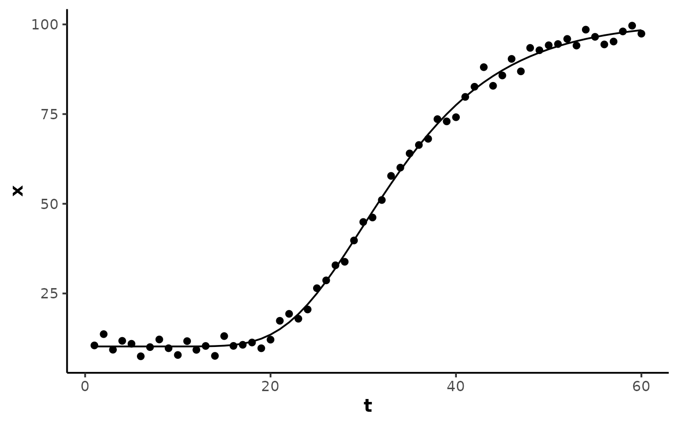
## create a Gompertz curve with random noise
set.seed(15)
t <- 1:60
x <- gompertz(t, A = 10, B = 100, xmid = 30, slope = 4) +
    rnorm(length(t), 0, 2)
data <- data.frame(t, x)

## fit with the self-starting wrapper
model <- nls(x ~ SSgompertz(t, A, B, xmid, slope), data = data)
summary(model)
#> 
#> Formula: x ~ SSgompertz(t, A, B, xmid, slope)
#> 
#> Parameters:
#>        Estimate Std. Error t value Pr(>|t|)    
#> A      10.23048    0.43131   23.72   <2e-16 ***
#> B     100.77389    0.84867  118.74   <2e-16 ***
#> xmid   29.92865    0.17117  174.85   <2e-16 ***
#> slope   4.01621    0.09135   43.96   <2e-16 ***
#> ---
#> Signif. codes:  0 ‘***’ 0.001 ‘**’ 0.01 ‘*’ 0.05 ‘.’ 0.1 ‘ ’ 1
#> 
#> Residual standard error: 1.811 on 56 degrees of freedom
#> 
#> Number of iterations to convergence: 4 
#> Achieved convergence tolerance: 1.076e-06
#> 

y <- predict(model, data)

# \donttest{
    if (requireNamespace("ggplot2", quietly = TRUE)) {
        ggplot2::ggplot(data, ggplot2::aes(t, x)) +
            theme_mnirs() +
            ggplot2::geom_point() +
            ggplot2::geom_line(ggplot2::aes(y = y))
    }

# }