Filter a data frame — filter

Apply digital filtering/smoothing to numeric vector data within a data frame using either:

A cubic smoothing spline.
A Butterworth digital filter.
A simple moving average.

Usage

filter_mnirs(
  data,
  nirs_channels = NULL,
  time_channel = NULL,
  method = c("smooth_spline", "butterworth", "moving_average"),
  na.rm = FALSE,
  verbose = TRUE,
  ...
)

Arguments

data

A data frame of class "mnirs" containing time series data and metadata.

nirs_channels

A character vector giving the names of mNIRS columns to operate on. Must match column names in data exactly.

If NULL (default), the nirs_channels metadata attribute of data is used.

time_channel

A character string giving the name of the time or sample column. Must match a column name in data exactly.

If NULL (default), the time_channel metadata attribute of data is used.

method

A character string indicating how to filter the data (see Details).

"smooth_spline": Fits a cubic smoothing spline.
"butterworth": Uses a centred Butterworth digital filter.
"moving_average": Uses a centred moving average filter.

na.rm

Logical; default is FALSE, propagates any NAs to the returned vector. If TRUE, ignores NAs and processes available valid samples within the local window. May return errors or warnings. (see Details).

verbose

Logical. Default is TRUE. Will display or silence (if FALSE) warnings and information messages helpful for troubleshooting. A global default can be set via options(mnirs.verbose = FALSE).

...

Additional method-specific arguments must be specified (see Details).

Value

A tibble of class "mnirs" with metadata available with attributes().

Details

filtering method

`method = "smooth_spline"`

Applies a non-parametric cubic smoothing spline from stats::smooth.spline(). Smoothing is defined by the parameter spar, which can be left as NULL and automatically determined via penalised log likelihood. This usually works well for responses occurring on the order of minutes or longer. spar can be specified typically, but not necessarily, in the range spar = [0, 1].

Additional arguments (...) accepted when method = "smooth_spline":

spar: A numeric smoothing parameter passed to stats::smooth.spline(). If NULL (default), automatically determined via penalised log likelihood.

`method = "butterworth"`

Applies a centred (two-pass symmetrical) Butterworth digital filter from signal::butter() and signal::filtfilt().

Filter type defines how the desired signal frequencies are either passed or rejected from the output signal. Low-pass and high-pass filters allow only frequencies lower or higher than the cutoff frequency, respectively to be passed through to the output signal. Stop-band defines a critical range of frequencies which are rejected from the output signal. Pass-band defines a critical range of frequencies which are passed through as the output signal.

The filter order (number of passes) is defined by order, typically in the range order = [1, 10]. Higher filter order tends to capture more rapid changes in amplitude, but also causes more distortion around those change points in the signal. General advice is to use the lowest filter order which sufficiently captures the desired rapid responses in the data.

The critical (cutoff) frequency can be defined by W, a numeric value for low-pass and high-pass filters, or a two-element vector c(low, high) defining the lower and upper bands for stop-band and pass-band filters. W represents the desired fractional cutoff frequency in the range W = [0, 1], where 1 is the Nyquist frequency, i.e., half the sample_rate of the data in Hz.

Alternatively, the cutoff frequency can be defined by fc and sample_rate together. fc represents the desired cutoff frequency directly in Hz, and sample_rate is the sample rate of the recorded data in Hz. Where W = fc / (sample_rate / 2).

Only one of either W or fc should be defined. If both are defined, W will be preferred over fc.

Additional arguments (...) accepted when method = "butterworth":

order: An integer for the filter order (default 2).
W: A numeric fractional cutoff frequency within [0, 1]. One of either W or fc must be specified.
fc: A numeric absolute cutoff frequency in Hz. Used with sample_rate to compute W.
sample_rate: A numeric sample rate in Hz. Will be taken from metadata or estimated from time_channel if not defined.
type: A character string specifying filter type, one of: c("low", "high", "stop", "pass") ("low" is the default).
edges: A character string specifying the edge padding, one of: c("rev", "rep1", "none") ("rev" is the default). See filter_butter().

`method = "moving_average"`

Applies a centred (symmetrical) moving average filter in a local window, defined by either width as the number of samples around idx between [idx - floor(width/2), idx + floor(width/2)]. Or by span as the timespan in units of time_channel between [t - span/2, t + span/2].

Additional arguments (...) accepted when method = "moving_average":

width or span: Either an integer number of samples, or a numeric time duration in units of time_channel within the local window. One of either width or span must be specified.
partial: Logical; FALSE by default, only returns values where a full window of valid (non-NA) samples are available. If TRUE, ignores NA and allows calculation over partial windows at the edges of the data.

Missing values

Missing values (NA) in nirs_channels will cause an error for method = "smooth_spline" or "butterworth", unless na.rm = TRUE. Then NAs will be ignored and passed through to the returned data.

For method = "moving_average", na.rm controls whether NAs within each local window are either propagated to the returned vector when na.rm = FALSE (the default), or ignored before processing if na.rm = TRUE.

Examples

## read example data and clean for outliers
data <- read_mnirs(
    file_path = example_mnirs("moxy_ramp"),
    nirs_channels = c(smo2 = "SmO2 Live"),
    time_channel = c(time = "hh:mm:ss"),
    verbose = FALSE
) |>
    replace_mnirs(
        invalid_values = c(0, 100),
        outlier_cutoff = 3,
        width = 10,
        verbose = FALSE
    )

data
#> # A tibble: 2,203 × 2
#>     time  smo2
#>    <dbl> <dbl>
#>  1 0        54
#>  2 0.400    54
#>  3 0.960    54
#>  4 1.51     54
#>  5 2.06     54
#>  6 2.61     54
#>  7 3.16     54
#>  8 3.71     57
#>  9 4.26     57
#> 10 4.81     57
#> # ℹ 2,193 more rows

data_filtered <- filter_mnirs(
    data,                   ## blank channels will be retrieved from metadata
    method = "butterworth", ## Butterworth digital filter is a common choice
    order = 2,              ## filter order number
    W = 0.02,               ## filter fractional critical frequency `[0, 1]`
    type = "low",           ## specify a "low-pass" filter
    na.rm = TRUE            ## explicitly ignore NAs
)

## note the smoothed `smo2` values
data_filtered
#> # A tibble: 2,203 × 2
#>     time  smo2
#>    <dbl> <dbl>
#>  1 0      54.4
#>  2 0.400  54.4
#>  3 0.960  54.4
#>  4 1.51   54.4
#>  5 2.06   54.4
#>  6 2.61   54.4
#>  7 3.16   54.4
#>  8 3.71   54.4
#>  9 4.26   54.4
#> 10 4.81   54.4
#> # ℹ 2,193 more rows

# \donttest{
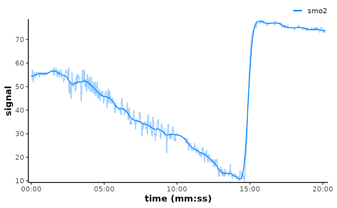
    if (requireNamespace("ggplot2", quietly = TRUE)) {
        ## plot filtered data and add the raw data back to the plot to compare
        plot(data_filtered, time_labels = TRUE) +
            ggplot2::geom_line(
                data = data,
                ggplot2::aes(y = smo2, colour = "smo2"), alpha = 0.4
            )
    }

# }