Processing Data with {mnirs}

Introduction

Modern wearable muscle near-infrared spectroscopy (mNIRS) devices make it extremely easy to collect local muscle oxygenation data during exercise. The real challenge comes with deciding how to filter, process, and interpret those data.

mnirs aims to provide standardised, reproducible methods for cleaning, filtering, and processing data, helping practitioners detect meaningful signals from noise and improve confidence in our interpretations and applications.

In this vignette we will demonstrate how to:

Read data files exported from various wearable mNIRS devices and import multiple mNIRS channels into a standard data frame with metadata.
Detect and replace local outlier and invalid values.
Resample (up- or down-sample) to match the sample rate of other recording devices.
Interpolate and fill across missing data.
Apply digital filtering to optimise signal-to-noise for the responses being observed in our data.
Shift and rescale data with multiple mNIRS channels, to modify signal dynamic range and absolute or relative scaling.
Save the filtered data to file with reproducible metadata for further analysis.

Read Data From File

We will read an example data file with two NIRS channels from an incremental ramp cycling assessment recorded with Moxy muscle oxygen monitor.

Example mNIRS Data Files

A few example data files are included in the mnirs package and can be accessed … <under development>

First, we load in the mnirs package and any other required libraries.

mnirs can also be installed with devtools::install_github("jemarnold/mnirs").

library(dplyr) ## load for data wrangling
library(ggplot2) ## load for plotting
library(mnirs) 
# devtools::install_github("jemarnold/mnirs") ## install development version

Specify file path

file_path: We should specify the location of our data file. e.g. r("C:\myfolder\my_file.xlsx") or "./my_file.xlsx". Or we can read in one of the included mnirs example data files.

file_path <- system.file("extdata", "moxy_ramp.xlsx", package = "mnirs")

Now we can read the data file with the read_data() function. This function will take in raw NIRS data exported from a device, and return a data frame with the NIRS channels we specify. See ?read_data for more details.

Specify channel names

We need to tell the function what channel names to look for, to identify our data table in the file. The data table may not be at the very top of the file, so these column names can be anywhere in the file.

nirs_channels: At minimum, we need one channel name defined for NIRS data.
time_channel: Typically, we will also specify a channel for the time or sample number of each observation.
event_channel: We can specify a channel to indicate laps or specific events in the dataset.

These names should be in quotations and exactly match the column headers in the file (case- and special character-sensitive). Multiple columns can be accepted for nirs_channels. We can rename these columns when importing our data in the format:

nirs_channels = c(new_name1 = "file_column_name1", 
                  new_name2 = "file_column_name2")

Other `read_data()` options

sample_rate: The sample rate of the NIRS recording can be specified if known, as number of samples per second, in Hz. If left blank, the function will estimate the sample rate from time_channel.
time_to_numeric: If time_channel is in a date-time format (e.g. hh:mm:ss), we can convert this to numeric with numeric_time = TRUE. The numeric time values will be re-sampled to start from zero.
time_from_zero: If the time_channel begins at a non-zero numeric value, it can be re-sampled to start from zero by using time_from_zero = TRUE.
keep_all: Once the data table in the file is identified, the default is to return only the column names explicitly specified above. If we want to return all columns in the data table, we can set keep_all = TRUE.
verbose: Finally, the function may return warnings or messages, for example if there are duplicate values in time_channel which may indicate a recording issue. These informative messages can be useful for data validation, but can be silenced with verbose = TRUE. Failure/abort error messages will always be returned.

data_raw <- read_data(file_path,
                      nirs_channels = c(smo2_left = "SmO2 Live",
                                        smo2_right = "SmO2 Live(2)"),
                      time_channel = c(time = "hh:mm:ss"),
                      event_channel = c(lap = "Lap"),
                      sample_rate = 2, ## we know this file is recorded at 2 samples per second
                      time_to_numeric = TRUE, ## to convert the date-time string to numeric
                      keep_all = FALSE, ## to keep the returned data frame clean
                      verbose = TRUE) ## show warnings & messages, but ignore them for now
#> Warning: `time_channel = time` has non-sequential or repeating values. Consider using
#> `resample_data()`.
#> ℹ Investigate at "time = 211.99, 211.99, 211.99, 1184, and 1184".

## ignore the Warning about repeated samples here for now

data_raw
#> # A tibble: 2,203 × 4
#>     time   lap smo2_left smo2_right
#>    <dbl> <dbl>     <dbl>      <dbl>
#>  1  0        1        54         68
#>  2  0.4      1        54         68
#>  3  0.96     1        54         68
#>  4  1.51     1        54         66
#>  5  2.06     1        54         66
#>  6  2.61     1        54         66
#>  7  3.16     1        54         66
#>  8  3.71     1        57         67
#>  9  4.26     1        57         67
#> 10  4.81     1        57         67
#> # ℹ 2,193 more rows

Plot `mnirs.data`

We can easily visualise our newly imported data frame by calling plot(data_raw). This generic plot function will work as long as the metadata contains class = "mnirs.data" or "mnirs.kinetics" as we’ll see later.

## {mnirs} data can be plotted with a built in call to `plot()`
plot(data_raw)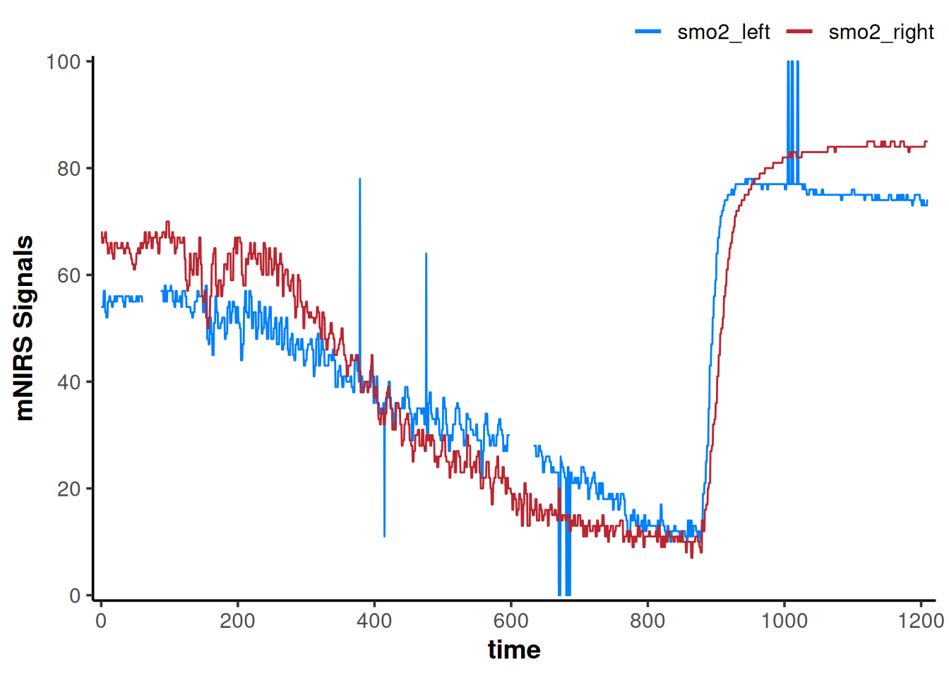

Metadata stored in `mnirs.data` data frames

Data frames read or processed by mnirs functions will return class = "mnirs.data" and contain metadata, which can be retrieved with attributes(data).

Instead of re-defining things like our channel names or sample rate, we can call them from the metadata. Certain mnirs functions will automatically retrieve metadata if present, without needing to explicitly call it at all.

nirs_channels <- attributes(data_raw)$nirs_channels
nirs_channels
#> [1] "smo2_left"  "smo2_right"

sample_rate <- attributes(data_raw)$sample_rate
sample_rate
#> [1] 2

Replace outliers, invalid values, and missing values

We can see some errors in the plot above, so let’s clean those up with some simple data wrangling steps, to prepare it for digital filtering and smoothing.

`replace_outliers()`

We can identify local outliers using a Hampel filter and replace them with the local median value. See ?replace_outliers for details.

x: These replace_* functions work on vector data; they take in a single data channel (x), apply processing to that channel, and return a vector of the processed channel data.
width: The number of samples (window) in which to detect local outliers. To define the window in seconds, multiply the desired number of seconds by the sample rate.
t0: The number of standard deviations outside of which are detected as outliers, defaulting to 3 (Pearson’s rule).
return: Indicates whether outliers should be replaced by the local “median” value or by “NA”. By default, this will return NA values which can be filled with replace_missing().

Note that with relatively low sample rates, such as this 2 Hz file, outlier filters may occasionally over-filter and ‘flatten’ sections of the data where the variance is already small.

`replace_invalid()`

Some NIRS devices or recording software can report specific invalid or nonsense values, such as c(0, 100, 102.3). These can be manually removed with replace_invalid(). See ?replace_invalid for details.

x: The numeric vector of the data channel to clean.
values: A vector of numeric values to be replaced.
width: The number of samples (window) in which the local median will be calculated. To define the window in seconds, multiply the desired number of seconds by the sample rate.
return: Indicates whether invalid values should be replaced by the local “median” value or by “NA”. By default, this will return NA values which can be filled with replace_missing().

`replace_missing()`

Finally, We can use replace_missing() to interpolate across missing data. Other fill methods are available, see ?replace_missing for details.

x: The numeric vector of the data channel to clean.
method: Specify the method for filling missing data. The default “linear” interpolation is usually sufficient.
maxgap: Specify the maximum number of consecutive NAs to fill. Any longer gaps will be left unchanged.

Subsequent processing & analysis steps may return errors when missing values are present. Therefore, it is a good habit to identify and deal with missing data early during data processing.

## simple data wrangling using {dplyr} from the {tidyverse}
data_cleaned <- data_raw |> 
    mutate(
        across(any_of(nirs_channels), ## apply a function across all of our `nirs_channels`
               \(.x) replace_outliers(x = .x, ## sequentially calls each of our `nirs_channels`
                                      width = 15, ## 15-sample window to detect local outliers
                                      return = "NA") ## we will fill these missing values later
        ),
        across(any_of(nirs_channels), 
               \(.x) replace_invalid(x = .x,
                                     values = c(0, 100), ## known invalid values
                                     return = "NA") ## with `NA` we do not need to specify `width`
        ),
        
        across(any_of(nirs_channels), 
               \(.x) replace_missing(x = .x,
                                     method = "linear", ## linear interpolation
                                     maxgap = Inf) ## interpolate across gaps of any length
        ),
    )

plot(data_cleaned)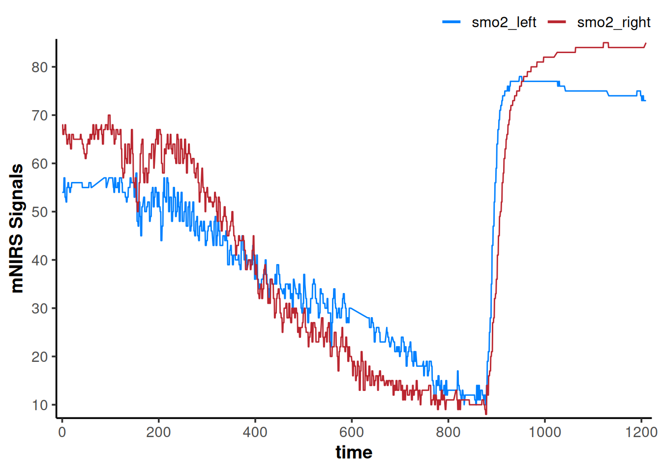

That got rid of all the obvious data issues.

Resample Data

Say we have NIRS data recorded at 50 Hz, but we are only interested in exercise responses on a time span of 5-minutes, and our other cycling power or heart rate data are only recorded at 1 Hz anyway. It may be easier and faster to down-sample our data to 1hz.

Alternatively, if we have something like high-frequency EMG data, we may want to up-sample our NIRS data to match samples. Although, we should be cautious with up-sampling as this can artificially inflate our confidence with certain modelling or processing methods.

`resample_data()` options

data: This function works on a data frame; it will take in a data frame, apply processing to all data channels, and return the processed data frame. Metadata will be passed to this function.
time_channel: If the data frame already has mnirs.data metadata, the time or sample channel will be detected automatically. Otherwise, we can define or overwrite it explicitly.
sample_rate: If the data frame already has mnirs.data metadata, the sample_rate will be detected automatically. Otherwise, we can define or overwrite it explicitly.
resample_rate: Specify the output sample rate we want to covert to, as a number of samples per second (Hz).
resample_time: Alternatively, we can specify the output as a number of seconds per sample to produce the same result.

This example dataset is already at relatively low sample rate, but let’s just see what it looks like if for some reason we wanted to down-sample further to 0.1 Hz (1 sample every 10 sec).

## `time_channel` and `sample_rate` will be read automatically from metadata
data_downsampled <- resample_data(data_cleaned,
                                  resample_time = 10, ## equal to `resample_rate = 0.1`
                                  na.rm = TRUE) ## interpolate across any missing data introduced by resampling
#> ℹ `sample_rate` = 2 Hz.
#> ℹ Output is resampled at 0.1 Hz.

## note the altered "time" values
data_downsampled
#> # A tibble: 121 × 4
#>     time   lap smo2_left smo2_right
#>    <dbl> <dbl>     <dbl>      <dbl>
#>  1     0     1      54         68  
#>  2    10     1      55         64  
#>  3    20     1      56         66  
#>  4    30     1      56         65  
#>  5    40     1      56         65  
#>  6    50     1      55         62  
#>  7    60     1      55         65  
#>  8    70     1      55.7       68  
#>  9    80     1      56.5       67.4
#> 10    90     1      57         68  
#> # ℹ 111 more rows

plot(data_downsampled)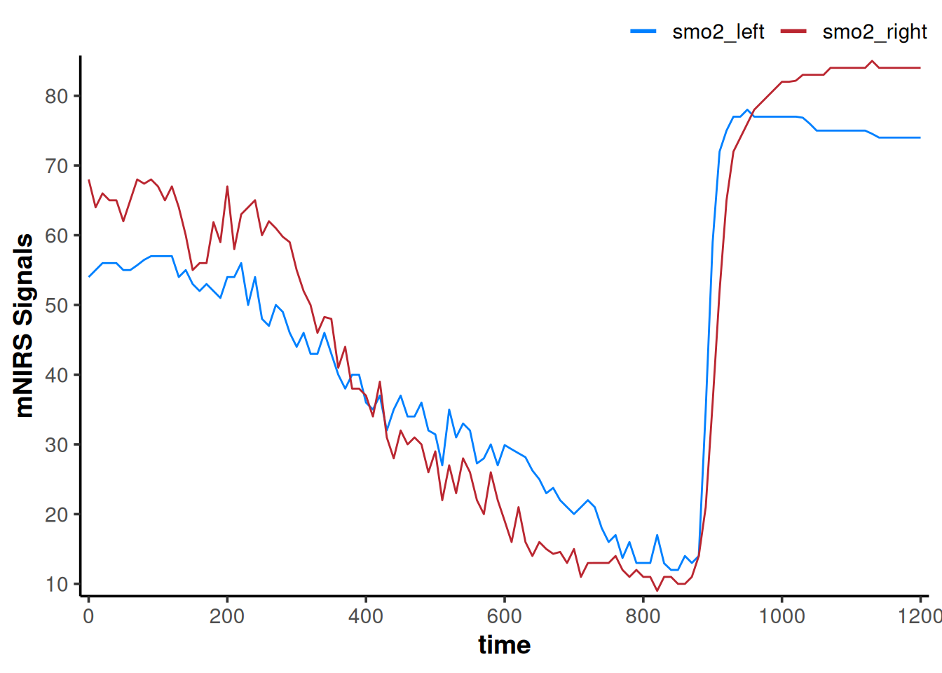

The data channels certainly look smoother. This is kind of like we have taken a 10-second moving average of the data.

But we have lost information by decreasing the number of samples. Our data frame now only has 121 rows, compared to the original 2203 rows.

Digital Filtering

If we want more precise control to improve our signal-to-noise ratio in our dataset without losing information, we should apply digital filtering to smooth the data.

Choosing a digital filter

There are a few digital filtering methods available. Which option is best will depend in large part on the sample rate of the data and the frequency of the response/phenomena being observed.

Choosing filter parameters is an important processing step to improve signal-to-noise ratio and enhance our subsequent interpretations. Over-filtering the data can introduce data artefacts which can negatively influence the signal analysis and interpretations just as much as an overly-noisy signal.

It is perfectly valid to choose a digital filter by empirically testing iterative filter parameters until the signal or response of interest is optimised for signal-to-noise ratio and minimal data artefacts.

The process of choosing a digital filter will be the topic of another vignette <currently under development>.

`filter_data()` methods

x: This function works on vector data; it takes in a single data channel (x), applies processing to that channel, and returns a vector of the processed channel data.

Smoothing-spline

method = "smooth-spline": A non-parametric smoothing spline is often quite good when first examining the data for longer time-span responses observed over multiple minutes. For faster occurring or repeated responses, a smoothing-spline may not work as well.

Butterworth digital filter

method = "butterworth": A Butterworth low-pass digital filter is probably the most common method used in mNIRS research (whether appropriately, or not). For certain applications such as identifying a signal with a known frequency (e.g. cycling/running cadence or heart rate), a pass-band or a different filter type may be better suited.

Moving average

method = "moving-average": The simplest smoothing method is a simple moving average applied over a specified number of samples. Commonly, this might be a 5- or 15-second centred moving average filter.

Apply the filter

Let’s try a Butterworth low-pass filter, and we’ll specify some empirically chosen filter parameters. See ?filter_data for further details on each of these filtering methods and their respective parameters.

data_filtered <- data_cleaned |> 
    mutate(
        across(any_of(nirs_channels),
               \(.x) filter_data(x = .x,
                                 method = "butterworth",
                                 type = "low",
                                 n = 2, ## see ?filter_data for details on filter parameters
                                 W = 0.02)
        )
    )

## we will add the non-filtered data back to the plot to compare
plot(data_filtered) +
    geom_line(data = data_cleaned, 
              aes(y = smo2_left, colour = "smo2_left"), alpha = 0.4) +
    geom_line(data = data_cleaned, 
              aes(y = smo2_right, colour = "smo2_right"), alpha = 0.4)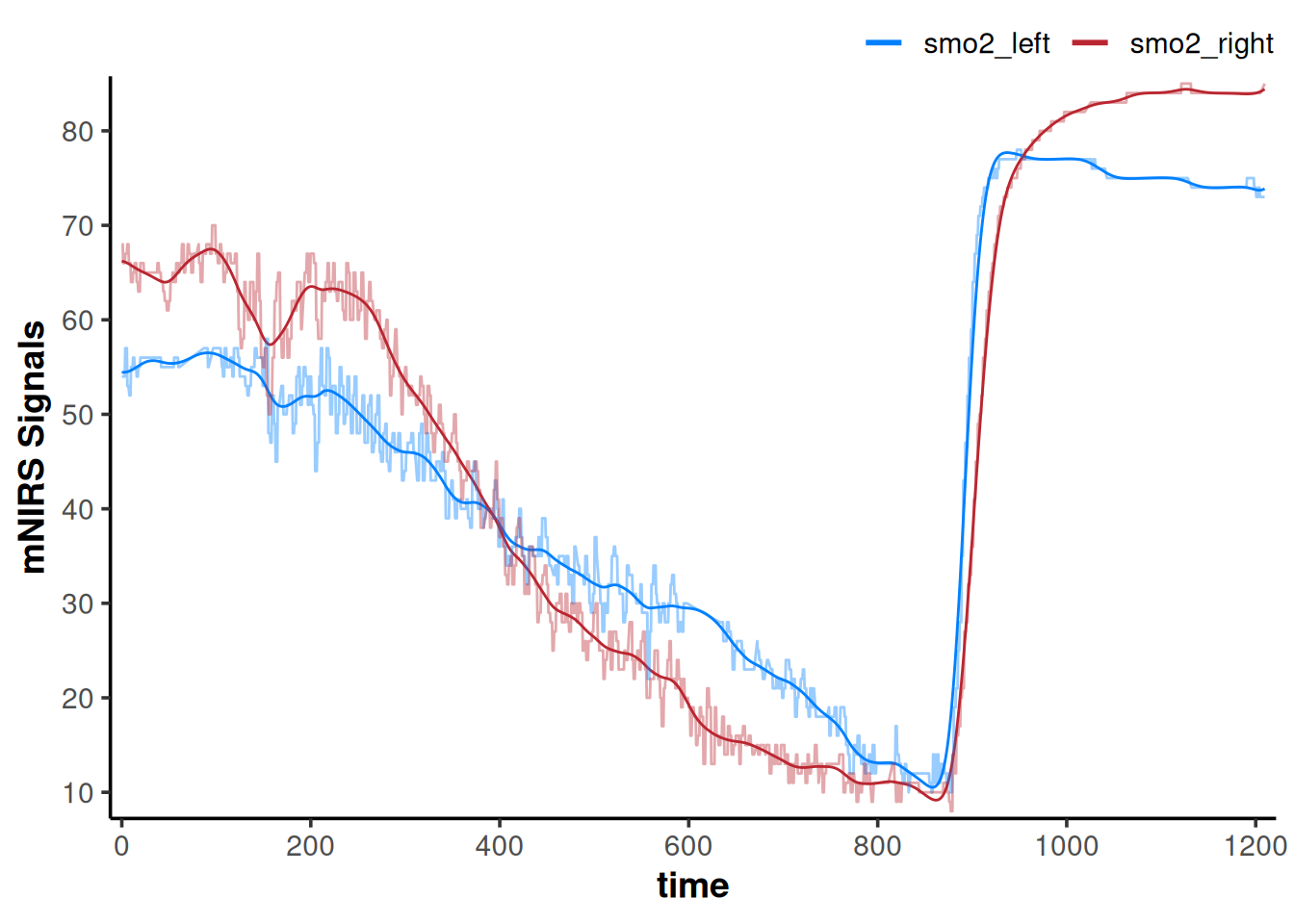

Shift and Rescale Data

We may need to adjust our data to normalise NIRS signal values across channels, or between individuals or trials, etc.

For example, we may want to set our mean baseline value to zero for all NIRS signals. Or we may want to compare signal kinetics (the rate of change or time course of a response) after rescaling to the same relative dynamic range.

These functions allow us to either shift values and preserve the dynamic range (the delta amplitude from minimum to maximum values) of our NIRS channels, or rescale the data to a new dynamic range.

We can do this on multiple NIRS channels and either modify or preserve the relative scaling between those channels.

`shift_data()` options

We may want to shift our data values while preserving the absolute dynamic range. See ?shift_data for details.

data: This function works on a data frame; it will take in a data frame, apply processing to all data channels, and return the processed data frame. Metadata will be passed to this function.
nirs_channels: A list specifying how we want the NIRS data channels to be grouped, to preserve relative scaling within groups. Listing each channel separately (e.g. list("A", "B", "C")) will shift each channel independently. The relative scaling between channels will be lost.

Grouping channels (e.g. list(c("A", "B"), c("C"))) will shift each group of channels together. The relative scaling between channels will be preserved within each group, but lost across groups.

nirs_channels must be grouped explicitly, even when mnirs.data metadata are present.
time_channel: If the data frame already has mnirs.data metadata, the time or sample channel will be detected automatically. Otherwise, we can define or overwrite it explicitly.
shift_to: The NIRS value to which the channels will be shifted.
position: Specifies how we want to shift the data; either shifting the “minimum”, “maximum”, or “first” sample(s) to the value specified by shift_to.
mean_samples: Specifies how many samples we want to average across when shifting to our new value specified above. The default mean_samples = 1 will shift a single value.
shift_by: An alternate way to specify, if we wanted to shift a data channel up by, say 10 units.

We have a 2-minute baseline for this dataset, so maybe we want to shift each NIRS channel so that the mean values of the 2-min baseline are equal to zero, which would then give us a change from baseline or "∇SmO[2]"

## un-group `nirs_channels` to shift each channel separately
as.list(nirs_channels)
#> [[1]]
#> [1] "smo2_left"
#> 
#> [[2]]
#> [1] "smo2_right"

data_shifted <- shift_data(data_filtered,
                           nirs_channels = as.list(nirs_channels),
                           shift_to = 0,
                           position = "first",
                           span = 120) ## shift the mean of the first 120 sec of data to zero

plot(data_shifted) +
    geom_hline(yintercept = 0, linetype = "dotted")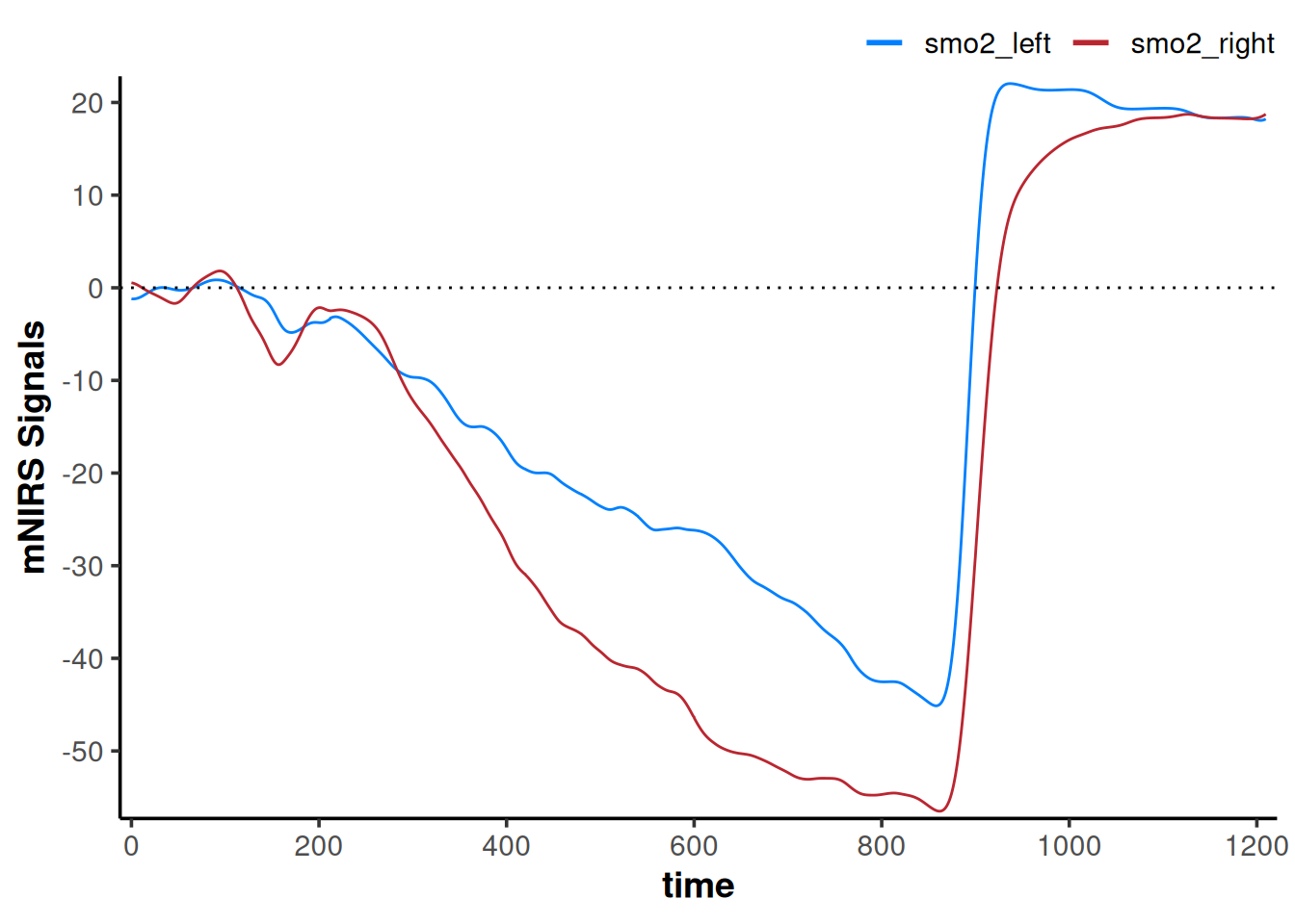

Now our interpretation may change; if we are assuming the baseline represents the same starting condition, our smo2_left signal does not deoxygenate as far as our smo2_right signal.

`rescale_data()` options

We may want to rescale our data to a new dynamic range. See ?rescale_data for details.

data: This function works on a data frame; it will take in a data frame, apply processing to all data channels, and return the processed data frame. Metadata will be passed to this function.
nirs_channels: A list specifying how we want the NIRS data channels to be grouped, to preserve relative scaling within groups. Must be grouped explicitly, even when mnirs.data metadata are present (see *shift_data()* above).
rescale_range: Specifies the new dynamic range, in the form c(minimum, maximum).

For example, if we are interested in comparing the rate of change within the ‘functional range’ of each NIRS signal during the exercise task, we may want to set them both to 0-100%.

data_rescaled <- rescale_data(data_filtered,
                              nirs_channels = as.list(nirs_channels), ## group `nirs_channels` to shift each channel separately
                              rescale_range = c(0, 100)) ## rescale to a 0-100% functional exercise range

plot(data_rescaled) +
    geom_hline(yintercept = c(0, 100), linetype = "dotted")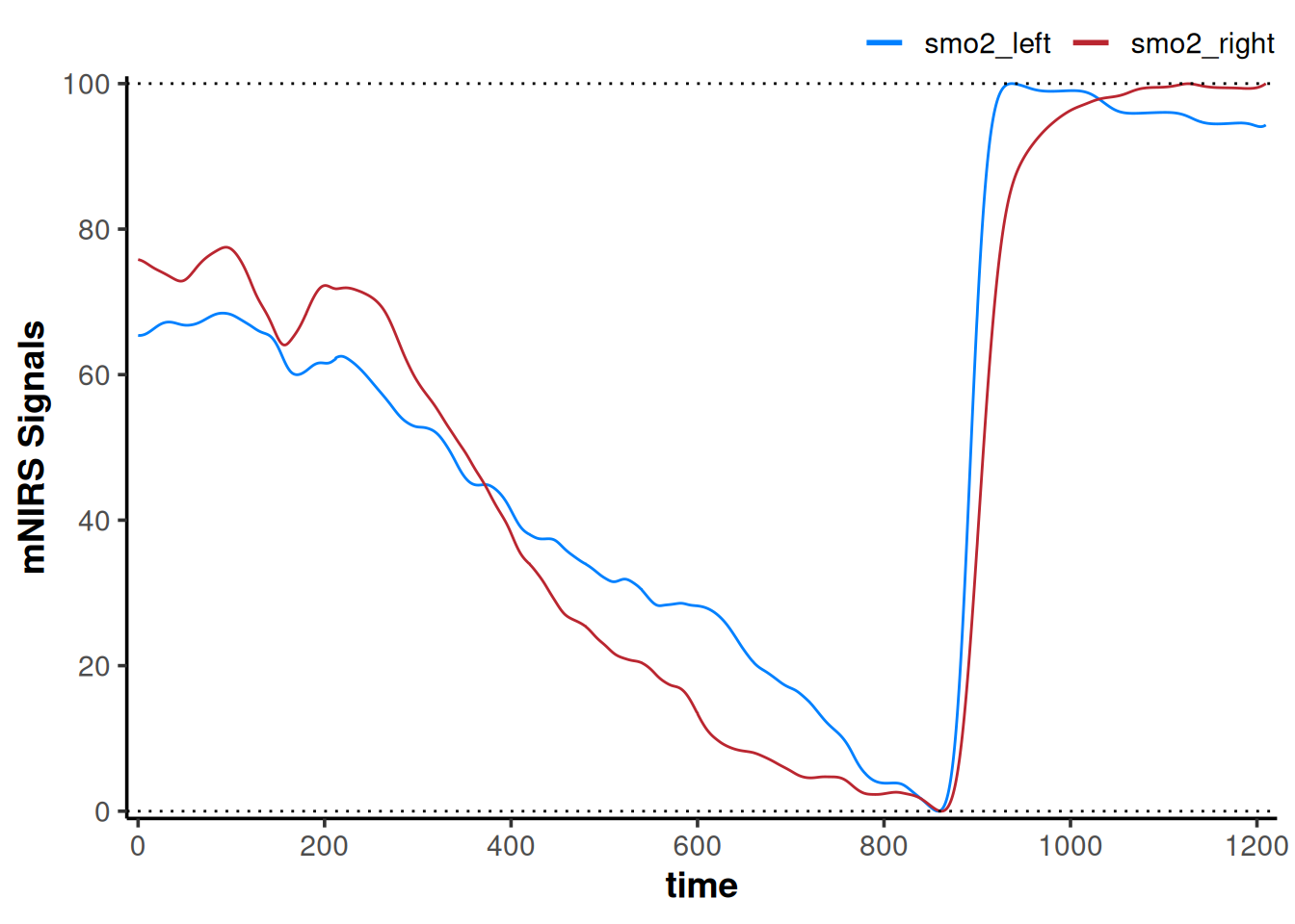

Here, our interpretation may be that smo2_left appears to deoxygenate slower to it’s fullest extent during incremental exercise, and reoxygenate faster compared to smo2_right.

Combined shift and rescale

What if we wanted to shift each NIRS signal to start from a mean 120-sec baseline at zero, then rescale the dynamic range of both signals grouped together, such that the highest and lowest values across both signals together are within 0-100?

## un-group `nirs_channels` to shift each channel separately
as.list(nirs_channels)
#> [[1]]
#> [1] "smo2_left"
#> 
#> [[2]]
#> [1] "smo2_right"

## then group `nirs_channels` to rescale together 
list(nirs_channels)
#> [[1]]
#> [1] "smo2_left"  "smo2_right"

data_rescaled <- data_filtered |> 
    ## shift the mean of the first 120 sec of each signal to zero
    shift_data(nirs_channels = as.list(nirs_channels),
               shift_to = 0,
               position = "first",
               span = 120) |> 
    ## then rescale the min and max of the grouped data to 0-100%
    rescale_data(nirs_channels = list(nirs_channels), 
                 rescale_range = c(0, 100))

plot(data_rescaled) +
    geom_hline(yintercept = c(0, 100), linetype = "dotted")

Now our interpretation might be that assuming the same starting baseline condition in both tissues, smo2_left preserves greater relative oxygenation during exercise and immediate recovery compared to smo2_right.