Reading and Cleaning Data with {mnirs}

Introduction

Modern wearable muscle near-infrared spectroscopy (mNIRS) devices make it extremely easy to collect local muscle oxygenation data during exercise. The real challenge comes with deciding how to clean, filter, and interpret those data.

mnirs package aims to provide standardised, reproducible methods for reading, cleaning, filtering, and processing NIRS data, helping practitioners detect meaningful signals from noise and improve confidence in our interpretations and applications.

In this vignette we will demonstrate how to:

Read data files exported from various wearable NIRS devices and import NIRS channels into a standard data frame with metadata, ready for further processing.
Plot and visualise data frames of class "mnirs.data".
Retrieve metadata stored with data frames of class "mnirs.data".
Detect and replace local outliers and invalid values.
Re-sample (up- or down-sample) to match the sample rate of other recording devices.
Interpolate and fill across missing data.
Apply digital filtering to optimise signal-to-noise ratio for the responses observed in our data.
Shift and rescale across multiple NIRS channels, to normalise signal dynamic range with absolute or relative scaling between muscle sites and NIRS channels.

Note

{mnirs} is currently . Functionality may change!

Stay updated on development and follow releases at github.com/jemarnold/mnirs.

Read Data From File

We will read an example data file with two NIRS channels from an incremental ramp cycling assessment recorded with Moxy muscle oxygen monitor.

First, install and load the {mnirs} package and other required libraries.

{mnirs} can be installed with remotes::install_github("jemarnold/mnirs").

# remotes::install_github("jemarnold/mnirs") ## install development version
library(dplyr) ## load for data wrangling
library(ggplot2) ## load for plotting
library(mnirs)

The first function to call will almost always be read_mnirs(). This is used to read data from .csv or .xls(x) files exported from common wearable mNIRS devices. It will extract and return the data table and metadata for further processing and analysis.

See read_mnirs() for more details.

`read_mnirs()`

file_path: Specify the location of the NIRS data file, including file extension. e.g. "./my_file.xlsx" or "C:/myfolder/my_file.csv".

Example Data Files

A few example data files are included in the {mnirs} package. Their file paths can be accessed with example_mnirs()

nirs_channels: At least one NIRS channel name must be specified from the data table in the file. Will accept multiple channel name inputs.
time_channel: A time or sample channel name from the data table must also be specified.
event_channel: Optionally we can specify a channel name which indicates events or laps in the data table.

These channel names are used to detect the data table within the file, and must match exactly with column headers in the file data table. We can rename these channels when reading data with the format:

nirs_channels = c(new_name1 = "original_name1", 
                  new_name2 = "original_name2")

sample_rate: The sample rate of the exported data file (in Hz) can either be specified explicitly, or it will be estimated from the time_channel in the data table itself.

This usually works well unless there is irregular sampling, or the time_channel is a count of samples rather than a time value, such as for data exported from Oxysoft. In this case, the function will recognise and read the correct sample rate from the file metadata. However, in most cases sample_rate should be defined explicitly if known.
add_timestamp: By default, if the time_channel is detected as date-time format (e.g.; hh:mm:ss), it will be converted to numeric time in seconds. This logical can specify to add or preserve a timestamp column of absolute date-time if detected in the file metadata, or relative timestamp if not.
zero_time: If time_channel values start at a non-zero value, this logical can specify to re-calculate time starting from zero. If the time_channel was converted from date-time format, it will always be re-calculated from zero.
keep_all: By default, only the channels specified above will be returned in the data table. This logical will return the entire data table as detected in the file. Blank/empty columns will be omitted and duplicated or invalid column names will be repaired.
verbose: This and other {mnirs} functions may return warnings and info messages which are useful for troubleshooting and data validation. This logical can be used to silence those messages.

## call an example mNIRS data file
file_path <- example_mnirs("moxy_ramp") 

data_table <- read_mnirs(
    file_path,
    nirs_channels = c(smo2_right = "SmO2 Live", ## identify and rename channels
                      smo2_left = "SmO2 Live(2)"),
    time_channel = c(time = "hh:mm:ss"), ## date-time format will be converted to numeric
    event_channel = "Lap",               ## assign event_channel without renaming
    sample_rate = NULL,                  ## sample_rate will be estimated from time column
    zero_time = TRUE,                    ## recalculate time values from zero
    add_timestamp = FALSE,               ## omit the date-time timestamp column
    keep_all = FALSE,                    ## return only the specified data channels
    verbose = TRUE                       ## show warnings & messages
)
#> ! Estimated `sample_rate` = 2 Hz.
#> ℹ Overwrite this with `sample_rate` = <numeric>.
#> Warning: ! `time_channel` has duplicated or irregular samples. Consider re-sampling with
#>   `mnirs::resample_mnirs()`.
#> ℹ Investigate at `time` = 211.99, 211.99, and 1184.

## ignore the warning about repeated samples for now ☝
## Note that sample_rate was estimated correctly at 2 Hz

data_table
#> # A tibble: 2,203 × 4
#>     time   Lap smo2_right smo2_left
#>    <dbl> <dbl>      <dbl>     <dbl>
#>  1  0        1         54        68
#>  2  0.4      1         54        68
#>  3  0.96     1         54        68
#>  4  1.51     1         54        66
#>  5  2.06     1         54        66
#>  6  2.61     1         54        66
#>  7  3.16     1         54        66
#>  8  3.71     1         57        67
#>  9  4.26     1         57        67
#> 10  4.81     1         57        67
#> # ℹ 2,193 more rows

Plot `mnirs.data`

mnirs.data can be easily visualised by calling plot(). This generic plot function uses the package ggplot2 and will work on data frames generated or read by {mnirs} functions where the metadata contain class = "mnirs.data".

## note the hidden plot option to display timestamp values as `hh:mm:ss`
plot(data_table, display_timestamp = TRUE)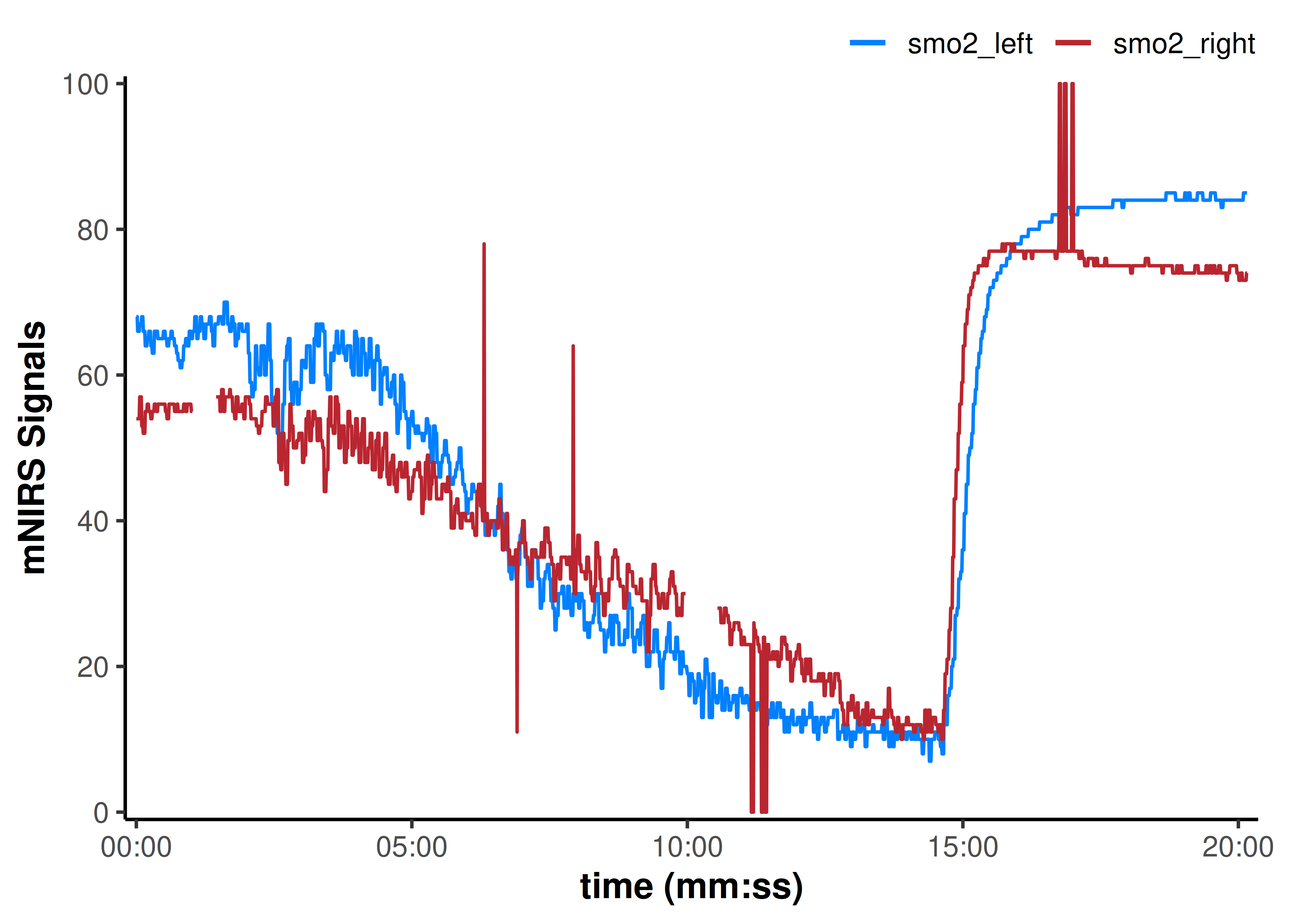

{mnirs} includes a custom ggplot2 theme and colour palette available with theme_mnirs() and palette_mnirs(). See those documentation references for more details.

Metadata stored in `mnirs.data` data frames

Data frames generated or read by {mnirs} functions will return class = "mnirs.data" and contain metadata, which can be retrieved with attributes(data).

Instead of re-defining values like our channel names or sample rate, certain {mnirs} functions will automatically retrieve them from metadata. They can always be overwritten manually in subsequent functions, or by using a helper function create_mnirs_data().

See create_mnirs_data() for more details about metadata.

## view metadata, omitting item two (a list of row numbers)
attributes(data_table)[-2]
#> $class
#> [1] "mnirs.data" "tbl_df"     "tbl"        "data.frame"
#> 
#> $names
#> [1] "time"       "Lap"        "smo2_right" "smo2_left" 
#> 
#> $nirs_channels
#> [1] "smo2_right" "smo2_left" 
#> 
#> $time_channel
#> [1] "time"
#> 
#> $event_channel
#> [1] "Lap"
#> 
#> $sample_rate
#> [1] 2

## define nirs_channels externally for later use
nirs_channels <- attr(data_table, "nirs_channels")
nirs_channels
#> [1] "smo2_right" "smo2_left"

## add nirs device to metadata
data_table <- create_mnirs_data(data_table, nirs_device = "Moxy")

## check that the added metadata is now present
attr(data_table, "nirs_device")
#> [1] "Moxy"

Replace local outliers, invalid values, and missing values

We can see some data issues in the plot above, so let’s clean those with a single data wrangling function replace_mnirs(), to prepare it for digital filtering and smoothing.

{mnirs} tries to include functions which work on vector data, and convenience wrapper functions which can be used on multiple specified columns in a data frame at once. Let’s explain the functionality of this data-wide function, and for more details about the vector-specific functions see replace_mnirs().

`replace_mnirs()`

data: Data-wide functions take in a data frame, apply processing to all channels specified, then return the processed data frame. mnirs.data metadata will be passed to and from this function./ / They are also pipe-friendly for Base R 4.1+ (|>) or magrittr (%>%) pipes to chain operations together.
nirs_channels: Specify which column names in data will be processed, i.e. the response variables. If not specified, these channels will be taken from mnirs.data metadata.
time_channels: The time channel can be specified, i.e. the predictor variable, or taken from mnirs.data metadata. If not specified or present in metadata, a sample index will be used instead. This can alter the results in unintended ways, and we suggest time_channel should be specified explicitly.
invalid_values: Optionally, invalid values can be specified for replacement, e.g. if a NIRS device exports 0 or 100 values when signal recording is lost. If left as NULL, no values will be replaced.
outlier_cutoff: Optionally, local outliers can be detected using a cutoff calculated from the local median value. A default value of 3 is recommended. If left as NULL, no outliers will be replaced.
width or span: Local outlier detection and median interpolation method occurs within a rolling local window specified by one of either width or span. width defines a number of samples on either side of the local index sample (idx), whereas span defines a range of time in units of time_channel (if it is specified) on either side of idx.
method: Missing data (NAs), invalid values, and local outliers specified above can be replaced via interpolation or fill methods; either "linear" interpolation, fill with local "median", or "locf" fill, which stands for “last observation carried forward”./ / NAs can be preserved with method = "NA". However, subsequent processing & analysis steps may return errors when NAs are present. Therefore, it is good practice to identify and deal with missing data early during data processing.
verbose: As above, a logical to toggle warnings and info messages.


data_cleaned <- replace_mnirs(
    data_table,
    nirs_channels = NULL,       ## default to all nirs_channels in metadata
    time_channel = NULL,        ## default to time_channel in metadata
    invalid_values = c(0, 100), ## known invalid values in the data
    outlier_cutoff = 3,         ## recommended default value
    width = 7,                  ## local window to detect local outliers and replace missing values
    method = "linear",          ## linear interpolation over `NA`s
)

plot(data_cleaned, display_timestamp = TRUE)

That cleaned up all the obvious data issues.

Resample Data

Say we have NIRS data recorded at 25 Hz, but we are only interested in exercise responses over a time span of 5-minutes, and our other heart rate data are only recorded at 1 Hz anyway. It may be easier and faster to work with our NIRS data down-sampled from 25 to 1 Hz.

Alternatively, if we have something like high-frequency EMG data, we may want to up-sample our NIRS data to match samples for analysis. Although, we should be cautious with up-sampling as this can artificially inflate our confidence with subsequent analysis or modelling methods.

`resample_mnirs()`

data: This function takes in a data frame, applies processing to all channels specified, then returns the processed data frame. mnirs.data metadata will be passed to and from this function.
time_channel & sample_rate: If the data contains mnirs.data metadata, these channels will be detected automatically. Or they can be specified explicitly.
resample_rate or resample_time: Resampling can be specified by one of either the resample_rate in number of samples per second (Hz), or the resample_time in number of seconds per sample (i.e. the inverse of each other).

The default resample_rate will re-sample back to the existing sample_rate of the data. This can be useful to average over irregular sampling resulting in unequal time values. Linear interpolation will be used to re-sample time_channel to round values of the sample_rate.

data_resampled <- resample_mnirs(
    data_cleaned,
    # time_channel = NULL,         ## taken from metadata
    # sample_rate = NULL,
    # resample_rate = sample_rate, ## the default will re-sample to sample_rate
    method = "linear",             ## default linear interpolation across any new samples
    verbose = TRUE                 ## will confirm the output sample rate
)
#> ℹ Output is resampled at 2 Hz.

## note the altered "time" values 👇
data_resampled
#> # A tibble: 2,419 × 4
#>     time   Lap smo2_right smo2_left
#>    <dbl> <dbl>      <dbl>     <dbl>
#>  1   0       1       54        68  
#>  2   0.5     1       54        68  
#>  3   1       1       54        67.9
#>  4   1.5     1       54        66.0
#>  5   2       1       54        66  
#>  6   2.5     1       54        66  
#>  7   3       1       54        66  
#>  8   3.5     1       55.9      66.6
#>  9   4       1       57        67  
#> 10   4.5     1       57        67  
#> # ℹ 2,409 more rows

This took care of the warning about irregular samples we saw earlier. Although nothing would be noticeable in the plot at this scale.

Use resample_mnirs() to smooth over irregular or skipped samples

If you are getting a warning from read_mnirs() about duplicated or irregular samples, resample_mnirs() can be used to restore regular sample rate and interpolate across skipped samples.

Digital Filtering

If we want to improve our signal-to-noise ratio in our dataset without losing information, we should apply digital filtering to smooth the data.

Choosing a digital filter

There are a few digital filtering methods available in {mnirs}. Which option is best for you will depend in large part on the sample rate of the data and the frequency of the response/phenomena being observed.

Choosing filter parameters is an important processing step to improve signal-to-noise ratio and enhance our subsequent interpretations. Over-filtering the data can introduce data artefacts which can negatively influence the signal analysis and interpretations just as much as trying to analyse overly-noisy raw data.

It is perfectly valid to choose a digital filter by empirically checking various filter parameters until the signal or response of interest appears to be visually optimised for signal-to-noise ratio and minimal data artefacts, to your satisfaction.

The process of choosing a digital filter will be the topic of another vignette <currently under development>.

`filter_mnirs()`

data: This function takes in a data frame, applies processing to all channels specified, then returns the processed data frame. mnirs.data metadata will be passed to and from this function.
nirs_channels, time_channel, & sample_rate: If the data contains mnirs.data metadata, these channels will be detected automatically. Or they can be specified explicitly.
na.rm: is an important argument which is left as FALSE by default. This will return an error if any missing data (NAs) are detected in the response variables (nirs_channels) being processed. Setting na.rm = TRUE will bypass these NAs and preserve them in the returned data frame, but this must be opted into explicitly in this function and elsewhere.

Smoothing-spline

method = "smooth-spline": The default non-parametric cubic smoothing spline is often a good first filtering option when examining the data for longer time span responses observed over multiple minutes. For more rapid and repeated responses, a smoothing-spline may not work as well.
spar: The smoothing parameter of the cubic spline can be determined automatically, or specified explicitly. See {stats::smooth.spline()}

Butterworth digital filter

method = "butterworth": A Butterworth low-pass digital filter (specified by type = "low") is probably the most common method used in mNIRS research (whether appropriately, or not). For certain applications such as identifying a signal with a known frequency (e.g. cycling/running cadence or heart rate), a pass-band or a different filter type may be better suited.
type: The filter type is specified as either c("low", "high", "stop", "pass").
n: The filter order number, specifying the number of passes the filter performs over the data.
W or fc: the cutoff frequency can be specified either as W; a fraction (between [0, 1]) of the Nyquist frequency, which is equal to half of the sample_rate of the data. Or as fc; the cutoff frequency in Hz.

For filtering vector data and more details about Butterworth filter parameters, see filter_butter().

Moving average

method = "moving-average": The simplest smoothing method is a moving average filter applied over a specified number of samples. Commonly, this might be a 5- or 15-second centred moving average.
width or span: Moving average filtering occurs within a rolling local window specified by one of either width or span. width defines a number of samples around the local index sample (idx), whereas span defines a range of time in units of time_channel (if it is specified) around idx.

For filtering vector data and more details about the moving average filter, see filter_moving_average()

Apply the filter

Let’s try a Butterworth low-pass filter, and we’ll specify some empirically chosen filter parameters for these data. See filter_mnirs() for further details on each of these filtering methods and their respective parameters.

data_filtered <- filter_mnirs(
    data_resampled,
    # nirs_channel = NULL,  ## taken from metadata
    # time_channel = NULL,
    # sample_rate = NULL,
    method = "butterworth", ## Butterworth digital filter is a common choice
    type = "low",           ## specify a low-pass filter
    n = 2,                  ## filter order number
    W = 0.02                ## filter fractional critical frequency
)

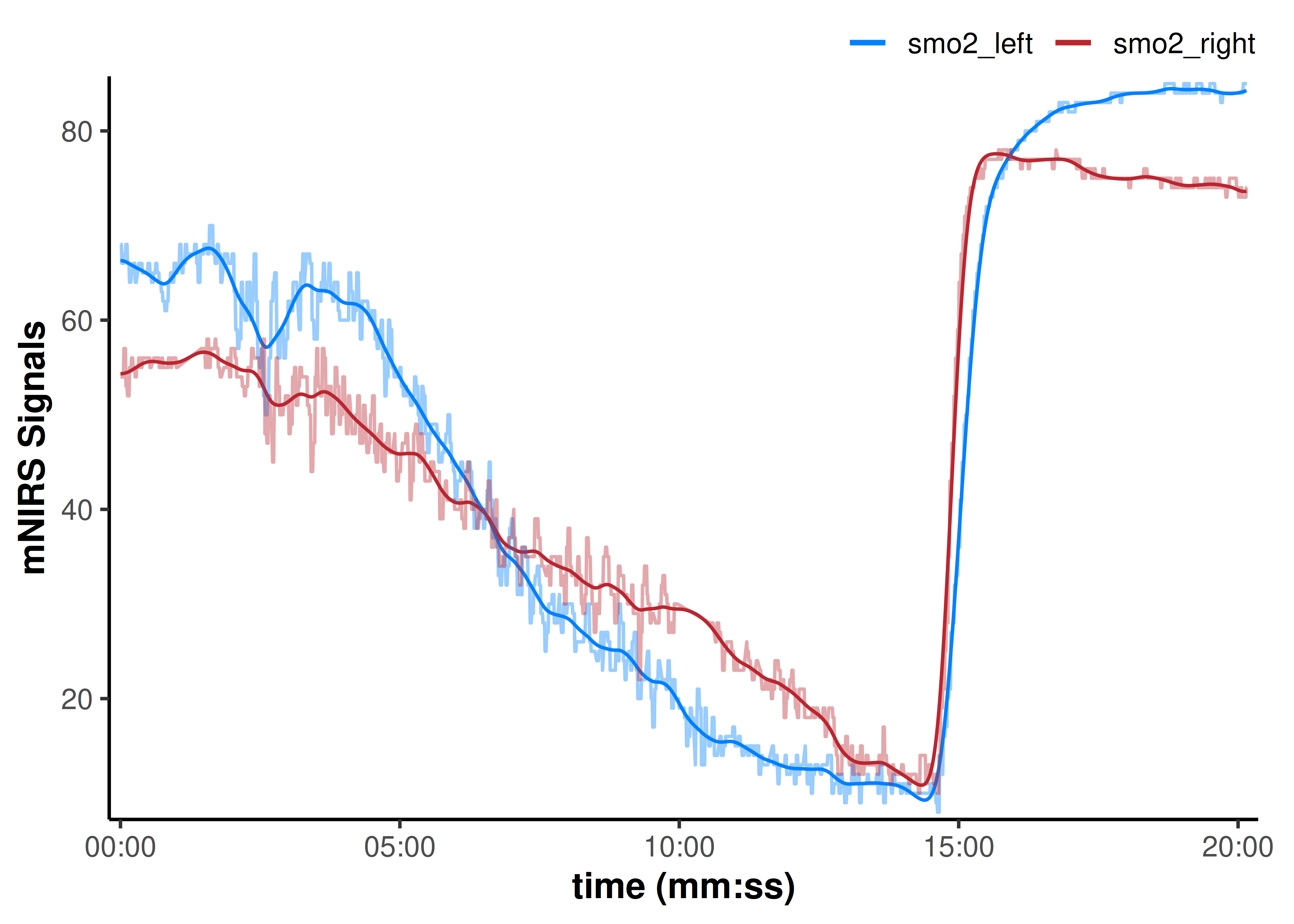
## we will add the non-filtered data back to the plot to compare
plot(data_filtered, display_timestamp = TRUE) +
    geom_line(
        data = data_cleaned, 
        aes(y = smo2_left, colour = "smo2_left"), alpha = 0.4
    ) +
    geom_line(
        data = data_cleaned, 
        aes(y = smo2_right, colour = "smo2_right"), alpha = 0.4
    )

Shift and Rescale Data

NIRS values are not measured on an absolute scale (even saturation %). Therefore, we may need to adjust or calibrate our data to normalise NIRS signal values between muscle sites, individuals, trials, etc.

For example, we may want to set our mean baseline value to zero for all NIRS signals at the start of a recording. Or we may want to compare signal kinetics (the rate of change or time course of a response) after rescaling signal amplitudes to the same dynamic range.

These functions allow us to either shift NIRS values up or down while preserving the dynamic range (the absolute amplitude from minimum to maximum values) of our NIRS channels, or rescale the data to a new dynamic range with larger or smaller amplitude.

We can group NIRS channels together to preserve the relative scaling among those channels.

`shift_mnirs()`

data: This function takes in a data frame, applies processing to all channels specified, then returns the processed data frame. mnirs.data metadata will be passed to and from this function.
nirs_channels: Channels can be grouped by providing a list (e.g. list(c("A", "B"), c("C"))) where each channel will be shifted to a common scale within group, and separate scales between groups. The relative scaling between channels will be preserved within each group, but lost across groups.

nirs_channels should be specified explicitly to ensure the intended grouping structure is defined. The default mnirs.data metadata will group all NIRS channels together.
time_channel: If the data contains mnirs.data metadata, this channels will be detected automatically. Or it can be specified explicitly
to or by: The shift amplitude can be specified by one of either shifting signals to a new value, or shifting signals by a fixed amplitude, given in units of the NIRS signals.
width or span: Shifting can be performed on the mean value within a window specified by one of either width or span. width defines a number of samples around the local index sample (idx), whereas span defines a range of time in units of time_channel around idx.

e.g. width = 1 will shift from the single minimum sample, whereas span = 1 would shift from the minimum mean value of all samples within one second.
position: Specifies how we want to shift the data; either shifting the “minimum”, “maximum”, or “first” sample(s).

For this data set, we could shift each NIRS channels so that the mean of the 2-minute baseline is equal to zero, which would then give us a change in deoxygenation from baseline during the incremental cycling protocol.

## our default *mnirs.data* nirs_channel will be grouped together
nirs_channels
#> [1] "smo2_right" "smo2_left"

## to shift each nirs_channel separately, the channels should be un-grouped
as.list(nirs_channels)
#> [[1]]
#> [1] "smo2_right"
#> 
#> [[2]]
#> [1] "smo2_left"

data_shifted <- shift_mnirs(
    data_filtered,
    nirs_channels = as.list(nirs_channels), ## un-grouped, as above
    to = 0,                                 ## NIRS values will be shifted to zero
    span = 120,                             ## shift the first 120 sec of data to zero
    position = "first")

plot(data_shifted, display_timestamp = TRUE) +
    geom_hline(yintercept = 0, linetype = "dotted")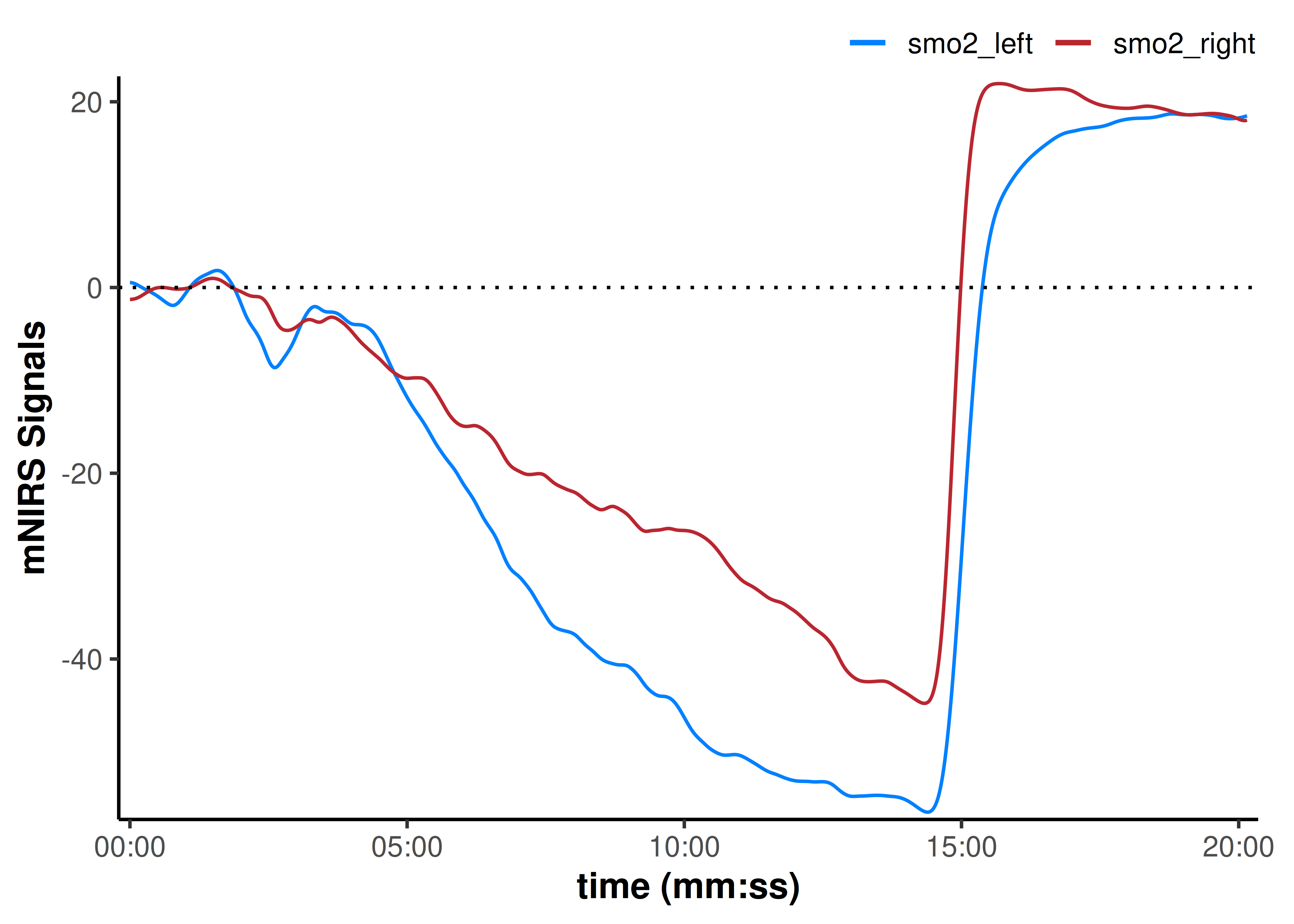

Before shifting, the ending (minimum) values for smo2_left and smo2_right were similar, but the starting baseline values were different. Whereas when we shift the baseline values to zero, we can see that the smo2_right signal has a smaller deoxygenation amplitude compared to the smo2_left signal.

We have to consider how our assumptions and processing decisions will influence our interpretations; by shifting both starting values, we are normalising for the starting condition of the two tissue sites and implicitly assuming the baseline represents the same starting condition in both legs. This may be appropriate when we are more interested in the relative change (delta) in each leg during an intervention or exposure (often referred to as "∇SmO[2]").

`rescale_mnirs()`

We may want to rescale our data to a new dynamic range, changing the units to a new amplitude.

data: This function takes in a data frame, applies processing to all channels specified, then returns the processed data frame. mnirs.data metadata will be passed to and from this function.
nirs_channels: Channels can be grouped by providing a list (e.g. list(c("A", "B"), c("C"))) where each channel will be rescaled to a common scale within group, and separate scales between groups. The relative scaling between channels will be preserved within each group, but lost across groups.

nirs_channels should be specified explicitly to ensure the intended grouping structure is defined. The default mnirs.data metadata will group all NIRS channels together.
range: Specifies the new dynamic range in the form c(minimum, maximum). For example, if we want to calibrate NIRS signals to the ‘functional range’ during an exercise task, we may want to rescale them both to 0-100%.

data_rescaled <- rescale_mnirs(
    data_filtered,
    nirs_channels = as.list(nirs_channels), ## un-group `nirs_channels` to rescale each channel separately
    range = c(0, 100))                      ## rescale to a 0-100% functional exercise range

plot(data_rescaled, display_timestamp = TRUE) +
    geom_hline(yintercept = c(0, 100), linetype = "dotted")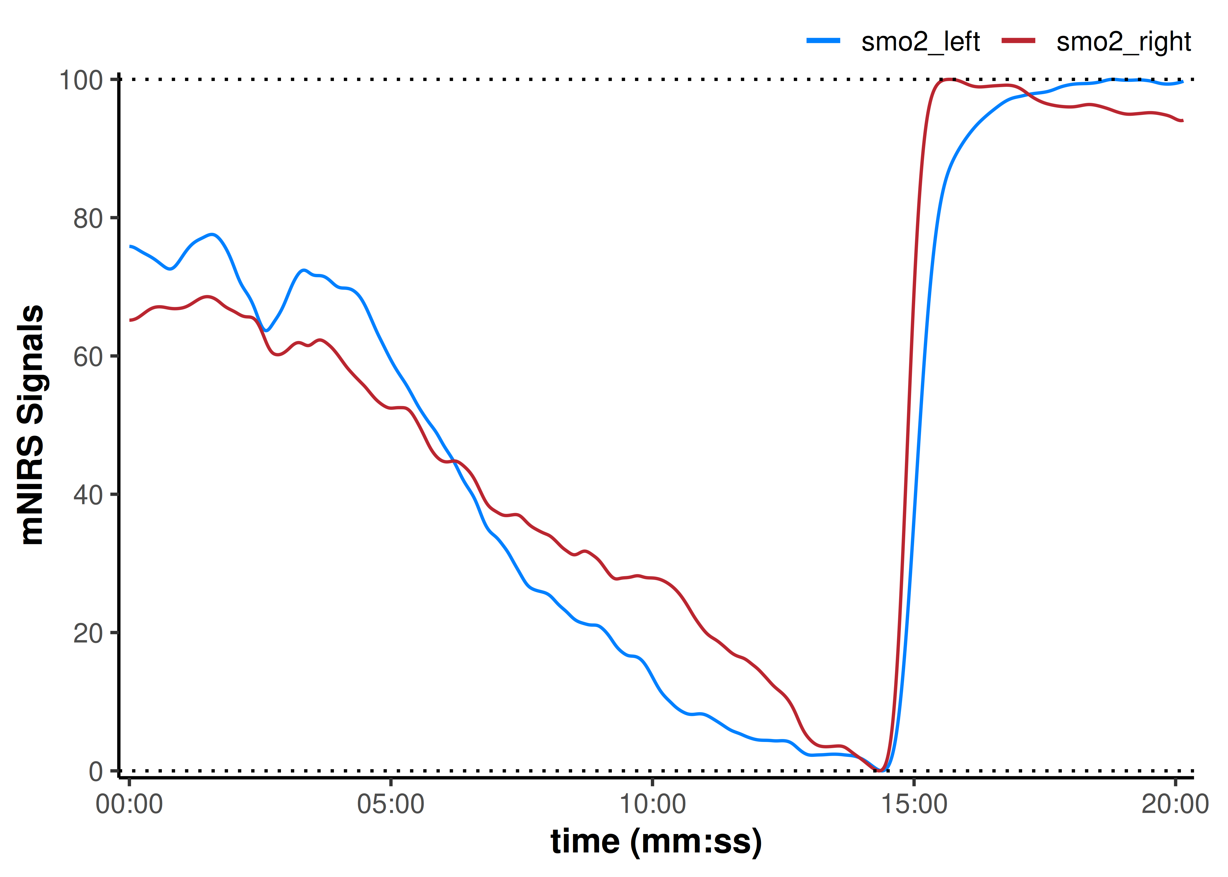

Here, our assumption is that during a maximal exercise task, the minimum and maximum values represent the functional capacity of the tissue being observed. So we normalise the functional dynamic range in each leg.

By normalising this way, the differences between smo2_left and smo2_right appear less pronounced than when the baselines were shifted to zero. Our interpretation may be that smo2_left appears to start at a slightly higher percent of it’s functional range, and deoxygenates faster toward it’s minimum. while smo2_right deoxygenates slightly slower during work, and reoxygenates slightly faster during recovery.

Combined shift and rescale

What if we wanted to shift each NIRS signal to start from a mean 120-sec baseline at zero, then rescale the dynamic range of both signals grouped together, such that the highest and lowest values across both signals together range from 0-100%?

This is also a good chance to demonstrate how functions can be piped together.

## un-group `nirs_channels` to shift each channel separately
as.list(nirs_channels)
#> [[1]]
#> [1] "smo2_right"
#> 
#> [[2]]
#> [1] "smo2_left"

## then group `nirs_channels` to rescale together 
list(nirs_channels)
#> [[1]]
#> [1] "smo2_right" "smo2_left"

## pipe (|>) data frame from one function to the next
data_rescaled <- data_filtered |> 
    ## shift the mean of the first 120 sec of each signal to zero
    shift_mnirs(
        nirs_channels = as.list(nirs_channels), ## un-grouped
        to = 0,
        position = "first",
        span = 120
    ) |> 
    ## then rescale the min and max of the grouped data to 0-100%
    rescale_mnirs(
        nirs_channels = list(nirs_channels), ## grouped
        range = c(0, 100)
    )

plot(data_rescaled, display_timestamp = TRUE) +
    geom_hline(yintercept = c(0, 100), linetype = "dotted")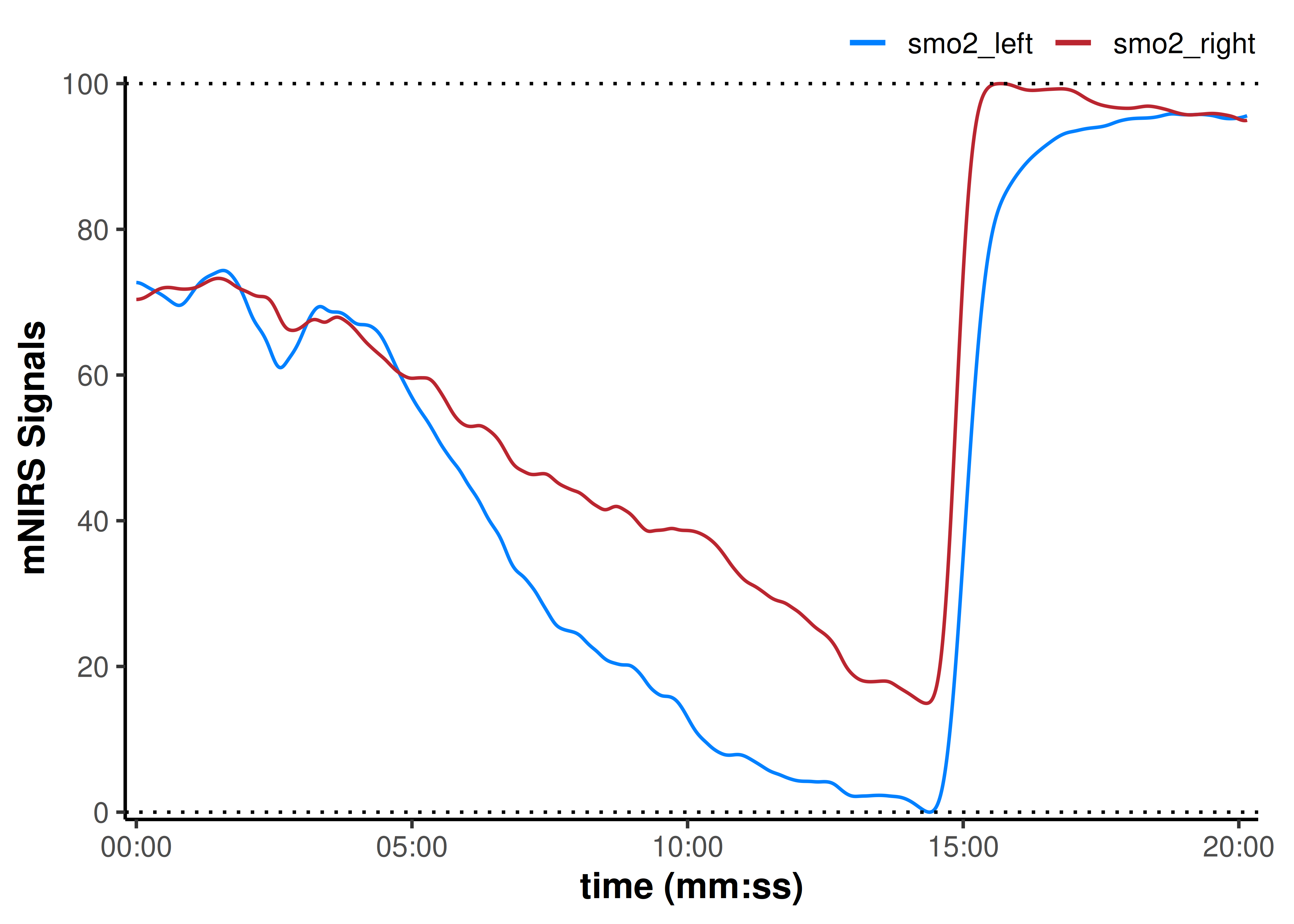

Our interpretation might now be that assuming the same starting baseline condition in both tissues, smo2_right deoxygenates less during exercise and recovers faster to a greater hyperaemic reperfusion, compared to smo2_left.

Signal Preparation

After the NIRS signal has been cleaned and filtered, it should be ready for further processing and analysis. {mnirs} is being developed to include functionality for processing discrete intervals and events, e.g. reoxygenation kinetics, slope calculations for post-occlusion microvascular responsiveness or critical oxygenation breakpoint.